4 Log Reg II

1. Count responses

Please load these libraries that you’ll need for this lab:

library(arm)
library(Sleuth3)
library(tidyverse)
library(vcdExtra)
library(magrittr)
library(datasets)

In this lab, We’ll cover the drop in deviance and deviance goodness of fit tests, and show how to perform them using R. We’ll also talk more about residuals from binomial logistic regression and about the dispersion parameter and over dispersion. Two additional topics are (1) a pathological (but not altogether rare) situation that can arise in logistic regression (2) using logistic regression to perform a test of the difference in two proportions.

2 Binomial logistic regression

In the previous lab, we introduced binary logistic regression in the context of a continuous explanatory variable (age). In this situation, each individual could, have had a unique combination of values of the explanatory variables. In practice,

due to rounding of ages to whole years, there were several explanatory variable combinations that occurred multiple times (this was why we had to jitter the plot of survival vs age). For those particular combinations of the explanatory variables (age/sex), we could count up the number of Donner party survivors and non-survivors so we’d have a count as the response, rather than a binary observations (survivors per age/sex?).

We are typically still inclined to think of the survival of individual Donner Party members, however; rather than in terms of the count of survivors out of the total number of members at each age-sex combination.

In this lab, we take a different perspective on logistic regression. We consider binary observations that are clustered into groups, where the counts of outcomes in each group are the natural measurements of interest. We consider each count to have a binomial distribution with some probability \(p\), and derive the log-odds from these binomial probabilities. Since a binomial \(p\) comes from an underlying Bernoulli \(p\) (or since a Bernoulli is a special case of a binomial), however, logistic regressions for binary outcomes and binomial counts are not fundamentally different beasts. They use the same model equations, they are fit with the same R function, they estimate the same parameters, and they rely on the same assumptions. Using binomial logistic regression when applicable, though, makes checking some of those assumptions more direct.

Aflatoxin data

In this lab we will continue with the ex2116 data from Sleuth3, introduced in lecture. Each of 20 tanks was stocked with fishes that had been exposed as embryos to one of 5 doses of a carcinogen. When the fishes were dissected a year later, the number of fishes that had developed liver tumors was recorded.

data(ex2116)
tumors <- ex2116
head(tumors)

Dose	Tumor	Total
0.010	9	87
0.010	5	86
0.010	2	89
0.010	9	85
0.025	30	86
0.025	41	86

Here we’ll add a column that records the number of fish in each tank which did not develop liver tumors, and a column that assigns a unique label to each of the 20 tanks. We’ll also add a column for log(Dose) and log(Dose)^2 since we used those as explanatory variables in the model you saw in the narrated lectures.

tumors %<>% mutate(Dose = Dose, Tumor = Tumor, NoTumor = Total - Tumor, TankID = factor(1:nrow(tumors)),logDose = log(Dose), logDose2 = log(Dose)^2)
head(tumors)

Dose	Tumor	Total	NoTumor	TankID	logDose	logDose2
0.010	9	87	78	1	-4.60517	21.20759
0.010	5	86	81	2	-4.60517	21.20759
0.010	2	89	87	3	-4.60517	21.20759
0.010	9	85	76	4	-4.60517	21.20759
0.025	30	86	56	5	-3.68888	13.60783
0.025	41	86	45	6	-3.68888	13.60783

We’ll also create a case-format version that records the binary status (tumor or not) for each of the 1739 individual fishes.

check code tumors_case$Outcome should be a factor

# The syntax dplyr::select() ensures that the select() function from the dplyr package is 
# used instead of the select() function from the MASS package, in case you still have MASS
# loaded in the library.
tumors_freq <- tumors %>% dplyr::select(-Total) %>%
 pivot_longer(Tumor:NoTumor,names_to="Outcome",values_to="Freq",cols_vary = "slowest") %>%
 mutate(Outcome=as.factor(Outcome))
tumors_case <- expand.dft(tumors_freq) %>%
 mutate(Outcome=as.factor(Outcome))
head(tumors_case)

Dose	TankID	logDose	logDose2	Outcome
0.01	1	-4.60517	21.20759	Tumor
0.01	1	-4.60517	21.20759	Tumor
0.01	1	-4.60517	21.20759	Tumor
0.01	1	-4.60517	21.20759	Tumor
0.01	1	-4.60517	21.20759	Tumor
0.01	1	-4.60517	21.20759	Tumor

(With most of the lab examples so far oriented around examples of death, discrimination, and disease, you might accuse us statisticians of attempting to usurp from economics the title of “dismal science”! (Economists think they’re pessimists. what they call “maximizing utility”, statisticians call “minimizing loss”). We promise nobody dies in the next lab. Probably.

Binary vs binomial

There are several equivalent ways of fitting a logistic regression model with glm() to data such as the ex2116 data. We will see why the fitting methods that preserve information about the counts within each tank are preferable for our purposes.

Modeling a binomial count for each tank

First, the response can be specified as a 2-column matrix containing counts of successes in the first column and counts of failures in the second.

mod1 <- glm(data = tumors, cbind(Tumor, NoTumor) ~ logDose + logDose2, family = "binomial")
summary(mod1)

Call:
glm(formula = cbind(Tumor, NoTumor) ~ logDose + logDose2, family = "binomial", 
    data = tumors)

Coefficients:
            Estimate Std. Error z value Pr(>|z|)    
(Intercept)  1.02921    0.49343   2.086  0.03699 *  
logDose     -1.03048    0.35743  -2.883  0.00394 ** 
logDose2    -0.39195    0.06136  -6.388 1.68e-10 ***
---
Signif. codes:  0 '***' 0.001 '**' 0.01 '*' 0.05 '.' 0.1 ' ' 1

(Dispersion parameter for binomial family taken to be 1)

    Null deviance: 667.195  on 19  degrees of freedom
Residual deviance:  26.048  on 17  degrees of freedom
AIC: 119.45

Number of Fisher Scoring iterations: 4

The response can also be specified as a vector of proportions of successes in each group, with the total in each group given through the weights argument:

mod2 <- glm(data = tumors, Tumor/Total ~ logDose + logDose2, weights = Total, family = "binomial")
summary(mod2)

Call:
glm(formula = Tumor/Total ~ logDose + logDose2, family = "binomial", 
    data = tumors, weights = Total)

Coefficients:
            Estimate Std. Error z value Pr(>|z|)    
(Intercept)  1.02921    0.49343   2.086  0.03699 *  
logDose     -1.03048    0.35743  -2.883  0.00394 ** 
logDose2    -0.39195    0.06136  -6.388 1.68e-10 ***
---
Signif. codes:  0 '***' 0.001 '**' 0.01 '*' 0.05 '.' 0.1 ' ' 1

(Dispersion parameter for binomial family taken to be 1)

    Null deviance: 667.195  on 19  degrees of freedom
Residual deviance:  26.048  on 17  degrees of freedom
AIC: 119.45

Number of Fisher Scoring iterations: 4

Be sure to verify that mod1 and mod2 are equivalent.

Modeling a binary outcome for each fish

We have converted the data to case format, where each row contains an individual binary outcome corresponding to an individual fish. These outcomes can be modeled directly, just as we saw with the (ungrouped) Donner data in Lab 3.

mod3 <- glm(data = tumors_case, Outcome ~ logDose + logDose2, family = "binomial")
summary(mod3)

Call:
glm(formula = Outcome ~ logDose + logDose2, family = "binomial", 
    data = tumors_case)

Coefficients:
            Estimate Std. Error z value Pr(>|z|)    
(Intercept)  1.02921    0.49341   2.086  0.03698 *  
logDose     -1.03048    0.35740  -2.883  0.00394 ** 
logDose2    -0.39195    0.06135  -6.388 1.68e-10 ***
---
Signif. codes:  0 '***' 0.001 '**' 0.01 '*' 0.05 '.' 0.1 ' ' 1

(Dispersion parameter for binomial family taken to be 1)

    Null deviance: 2395.8  on 1738  degrees of freedom
Residual deviance: 1754.7  on 1736  degrees of freedom
AIC: 1760.7

Number of Fisher Scoring iterations: 4

Make a quick comparison of the coefficient estimates from mod2 and mod3:

cbind(coefficients(mod2),coefficients(mod3))

                  [,1]      [,2]
(Intercept)  1.0292126  1.029213
logDose     -1.0304804 -1.030480
logDose2    -0.3919491 -0.391949

The two models give the same coefficient estimates, and you can also verify that the corresponding standard errors are the same. Therefore, in terms of inferences about the regression coefficients, treating the data as binary (one 0/1 outcome for each fish) or binomial (one count outcome for each tank) doesn’t seem to matter.

But, let’s remember that when we looked at the binomial logistic regression model in class, we noticed some over dispersion in the counts. We’ll first examine one more approach to modeling the binomial counts, and then turn to talking about the over dispersion.

Modeling as binomial counts within each Dose

Note that “TankID” is not a term in any of the models we fit above. The binomial logistic models treat the 4 tanks in each of the 5 dose groups as independent binomial observations. Within each Dose level, the 4 tanks are supposed to be draws from 4 independent binomial random variables, with potentially different \(n\) (different number of fish in each tank) but all with the same \(p\). In the binary logistic model, the tanks are ignored and the fish-level outcomes are treated as independent Bernoulli random variables, with a common \(p\) at each Dose. In either form, a single \(p\) applies to every fish in the Dose level, regardless of tank. Indeed, we can explicitly collapse across the tanks before fitting the model, without affecting any of the inferences:

(summed_tumor <- summarize(group_by(tumors, Dose, logDose, logDose2), sum(Tumor), sum(NoTumor)))

`summarise()` has grouped output by 'Dose', 'logDose'. You can override using
the `.groups` argument.

Dose	logDose	logDose2	sum(Tumor)	sum(NoTumor)
0.010	-4.605170	21.207592	25	322
0.025	-3.688880	13.607832	132	214
0.050	-2.995732	8.974412	226	127
0.100	-2.302585	5.301898	281	74
0.250	-1.386294	1.921812	286	52

Notice that we’ve now reduced the dataset down to five observations! And now we’ll fit the model to these summed responses:

mod4 <- glm(data = summed_tumor, cbind(`sum(Tumor)`, `sum(NoTumor)`) ~ logDose + logDose2, family = "binomial")
summary(mod4)

Call:
glm(formula = cbind(`sum(Tumor)`, `sum(NoTumor)`) ~ logDose + 
    logDose2, family = "binomial", data = summed_tumor)

Coefficients:
            Estimate Std. Error z value Pr(>|z|)    
(Intercept)  1.02921    0.49343   2.086  0.03699 *  
logDose     -1.03048    0.35743  -2.883  0.00394 ** 
logDose2    -0.39195    0.06136  -6.388 1.68e-10 ***
---
Signif. codes:  0 '***' 0.001 '**' 0.01 '*' 0.05 '.' 0.1 ' ' 1

(Dispersion parameter for binomial family taken to be 1)

    Null deviance: 641.234089  on 4  degrees of freedom
Residual deviance:   0.086879  on 2  degrees of freedom
AIC: 35.091

Number of Fisher Scoring iterations: 3

And compare coefficient estimates:

cbind(coefficients(mod2),coefficients(mod3),coefficients(mod4))

                  [,1]      [,2]       [,3]
(Intercept)  1.0292126  1.029213  1.0292126
logDose     -1.0304804 -1.030480 -1.0304804
logDose2    -0.3919491 -0.391949 -0.3919491

And once again you can verify that all of the corresponding standard errors are also the same. So what’s going on here, and which of these models is “the best one” to use?

Ok, so now what?!

The parameter estimates and standard errors are all identical. We reach the same conclusions from each model. But let’s look at the residual deviances for each of the models:

cbind(deviance(mod2),deviance(mod3),deviance(mod4))

         [,1]     [,2]       [,3]
[1,] 26.04806 1754.692 0.08687945

It’s also important to recognize that in mod2, mod3 and mod4, the sample sizes are n = 20, n = 1739 and n = 5, respectively. And, the null deviances for each model are also substantially different; again in order of mod2, mod3 and mod4 these are 667.20, 2395.84 and 641.23. The difference in deviance (the deviance accounted for by a model), however, is the same for every form of the model.

To see more plainly that the methods above are equivalent, we can view minimal summaries from each using the display() function from arm. The abbreviated output (compared to summary) facilitates comparison between several models on the same page.

# counts in tanks
display(mod2)

glm(formula = Tumor/Total ~ logDose + logDose2, family = "binomial", 
    data = tumors, weights = Total)
            coef.est coef.se
(Intercept)  1.03     0.49  
logDose     -1.03     0.36  
logDose2    -0.39     0.06  
---
  n = 20, k = 3
  residual deviance = 26.0, null deviance = 667.2 (difference = 641.1)

# binary outcomes per fish
display(mod3)

glm(formula = Outcome ~ logDose + logDose2, family = "binomial", 
    data = tumors_case)
            coef.est coef.se
(Intercept)  1.03     0.49  
logDose     -1.03     0.36  
logDose2    -0.39     0.06  
---
  n = 1739, k = 3
  residual deviance = 1754.7, null deviance = 2395.8 (difference = 641.1)

# counts in dose level ignoring tanks
display(mod4)

glm(formula = cbind(`sum(Tumor)`, `sum(NoTumor)`) ~ logDose + 
    logDose2, family = "binomial", data = summed_tumor)
            coef.est coef.se
(Intercept)  1.03     0.49  
logDose     -1.03     0.36  
logDose2    -0.39     0.06  
---
  n = 5, k = 3
  residual deviance = 0.1, null deviance = 641.2 (difference = 641.1)

All the same assumptions go into each of these ways of fitting the models, and all the same inferences come out. In particular, we are always assuming that once we know the Dose a fish received, knowing the particular tank in which that fish was housed cannot give us any more information about that fish’s chance of having a tumor – not even if we know that the fish came from a tank in which an especially large (or small) number of other fish got tumors, compared to other tanks within the same dose level. In the binomial-tank-counts model, this assumption reads like “every binomial within a dose level has the same \(p\).” In the binary-fish model, it reads “every Bernoulli within a dose level has the same \(p\).” In the binomial-dose-count model, it reads “the Bernoulli’s across all tanks within a dose must be independent.” We could call this the assumption of “irrelevant groups (tanks).”

If we have some grouping at all, however, we often suspect that this last assumption about independence is not sound. Fish in the same tank are expected to be more similar to one another than fish in different tanks. That is, we should not expect same binomial \(p\) in every tank, nor should we suppose that all the Bernoulli responses in a dose level are independent, regardless of tank.

In what follows, we will see that fitting the model in the “tank-count” binomial form, as opposed to per-fish binary form or the dose-count binomial form, is the way that will allow us to check whether the group-irrelevance of assumption is reasonable. We’ll see that not making this assumption comes with a steep price, and preview another technique that will sometimes allow us to avoid paying it.

3. Model fit and model comparison

In the binary logistic case, there was little we could do to directly assess model fit. You could try squinting at some residual plots, but that’s about it. The single binary outcomes just bounce around too much to say of anything about what the fitted line “should have done” at any given predictor value. It certainly should not chase every individual 1 or 0. To get some stability, you need to be able to put multiple observations within the same “bin”, so that you can say whether the proportion (or log-odds) in that bin is close to what the model predicts.

Empirical logits

The empirical logit is just the logit transformation applied to the proportion within a bin (this isn’t the log-odds of the probability within the bin, it’s just an estimate based on the observed proportion, hence “empirical”).

Remember the logit transformation of a proportion/probability is given by qlogis():

tumors

Dose	Tumor	Total	NoTumor	TankID	logDose	logDose2
0.010	9	87	78	1	-4.605170	21.207592
0.010	5	86	81	2	-4.605170	21.207592
0.010	2	89	87	3	-4.605170	21.207592
0.010	9	85	76	4	-4.605170	21.207592
0.025	30	86	56	5	-3.688880	13.607832
0.025	41	86	45	6	-3.688880	13.607832
0.025	27	86	59	7	-3.688880	13.607832
0.025	34	88	54	8	-3.688880	13.607832
0.050	54	89	35	9	-2.995732	8.974412
0.050	53	86	33	10	-2.995732	8.974412
0.050	64	90	26	11	-2.995732	8.974412
0.050	55	88	33	12	-2.995732	8.974412
0.100	71	88	17	13	-2.302585	5.301898
0.100	73	89	16	14	-2.302585	5.301898
0.100	65	88	23	15	-2.302585	5.301898
0.100	72	90	18	16	-2.302585	5.301898
0.250	66	86	20	17	-1.386294	1.921812
0.250	75	82	7	18	-1.386294	1.921812
0.250	72	81	9	19	-1.386294	1.921812
0.250	73	89	16	20	-1.386294	1.921812

empirical_logits <- with(tumors, qlogis(Tumor/Total))
empirical_logits

 [1] -2.15948425 -2.78501124 -3.77276094 -2.13350876 -0.62415431 -0.09309042
 [7] -0.78170058 -0.46262352  0.43363599  0.47378435  0.90078655  0.51082562
[13]  1.42946653  1.51787072  1.03889305  1.38629436  1.19392247  2.37157796
[19]  2.07944154  1.51787072

We plot the empirical logits against Dose to see the shape of the relationship we’re trying to capture on the log-odds scale, along with a loess smooth.

ggplot(data = tumors, aes(x = Dose, y = empirical_logits))+ 
 geom_jitter(width = 0.005, height = 0.01) + 
 geom_smooth(se = FALSE) +
 ggtitle("Empirical Logits vs Dose") 

`geom_smooth()` using method = 'loess' and formula = 'y ~ x'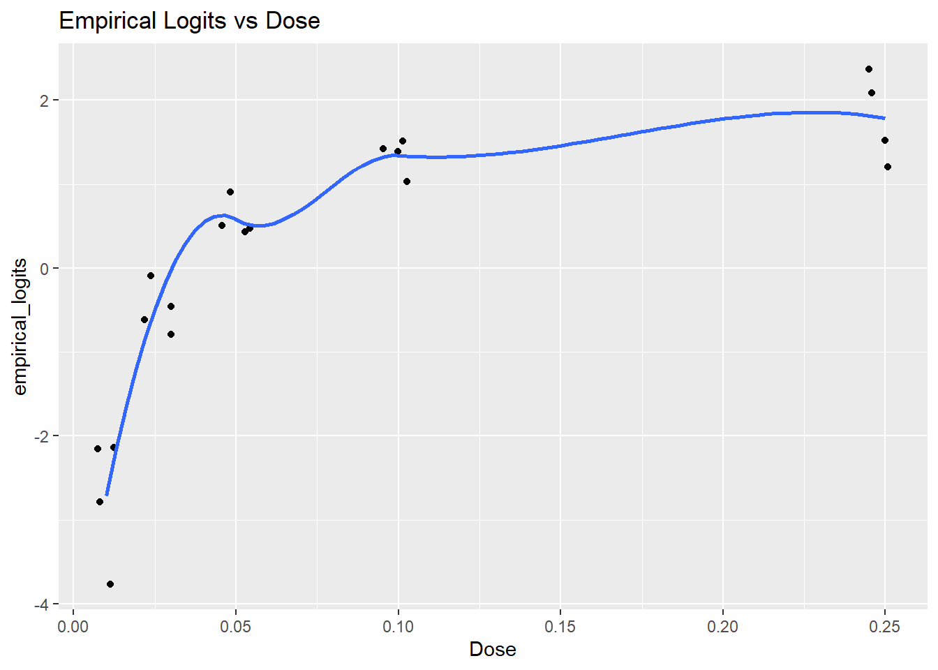

This appearance of a logarithmic relationship between the Dose and the logits prompts the a log-transformation of the dose to straighten it out (that is, it suggests that the odds of tumor are nearly linear in dose).

ggplot(data = tumors, aes(x = logDose, y = empirical_logits)) + 
 geom_jitter(width = 0.1, height = 0.1) + 
 geom_smooth(se = FALSE) +
 ggtitle("Empirical Logits vs log(Dose)")

`geom_smooth()` using method = 'loess' and formula = 'y ~ x'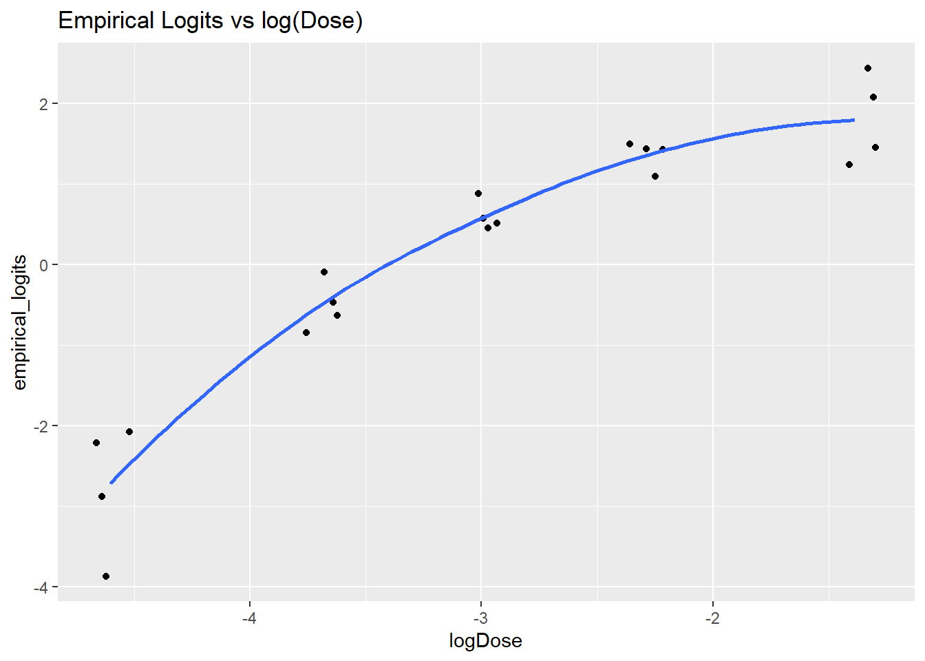

This plot suggests that a logistic regression model which includes both log(Dose) and log(Dose)^2 would be appropriate to capture the observed trend in the empirical logits. Unlike with binary logistic regression, the binomial model lets us measure the lack-of-fit to a proposed model, and compare the fit between models.

Deviance goodness of fit , lack of fit.

Recall that the deviance goodness of fit test compares a fitted model to a saturated model, or one in which there are as many parameters as there are data points. In these goodness of fit comparisons,

the null hypothesis corresponds to the fitted model (which is a reduced model relative to the saturated model), and the alternative hypothesis corresponds to the saturated model. Therefore, a small p-value indicating evidence for rejection of the fitted model in favor of the saturated model is evidence of lack of fit.

The LRstats() from vcdExtra function shows a convenient summary of the fits of one or more model objects.

mod5 <- glm(data = tumors, (Tumor/Total) ~ Dose, weights = Total, family = "binomial")
mod6 <- glm(data = tumors, (Tumor/Total) ~ logDose, weights = Total, family = "binomial")
mod7 <- glm(data = tumors, (Tumor/Total) ~ logDose + logDose2, weights = Total, family = "binomial")
LRstats(mod5, mod6, mod7)

	AIC	BIC	LR Chisq	Df	Pr(>Chisq)
mod5	368.4449	370.4364	277.04682	18	0.0000000
mod6	160.2947	162.2862	68.89661	18	0.0000001
mod7	119.4461	122.4333	26.04806	17	0.0735894

The LR Chisq is the residual deviance, which is the sum of the squared deviance residuals. For instance, for mod5, the residual deviance value of 277 comes can be obtained as

resid(mod5, type = 'deviance') %>% raise_to_power(2) %>% sum

[1] 277.0468

or as

mod5$deviance

[1] 277.0468

This quantity has an approximate chi-squared distribution if the model is correct, which is the basis for the deviance goodness of fit test. Pr(>Chisq) provides the p-value for this test. For mod6, let’s check that this is equivalent to doing this test “by hand,” using the residual deviance and residual df:

pchisq(mod6$deviance, df = mod6$df.residual, lower.tail = FALSE)

[1] 6.940025e-08

Each successive model shows a better fit, as evidenced by the successively larger p-values from the goodness of fit tests.

Drop-in-deviance test

Just a reminder that the drop in deviance test is different from the deviance goodness of fit test. Whereas the deviance goodness of fit test provides a comparison between a single fitted model and a saturated model, a drop in deviance test provides a way to compare two fitted models when one of those models is nested within the other one. Put another way, the drop in deviance test is a comparison between a reduced model (null hypothesis) and a full model (alternative hypothesis) and we use it in cases where the reduced model is reduced from (or nested in) the full model.

Using the models we have already fit, let’s use the anova() function to perform a drop in deviance test comparing a reduced model (only logDose included) to a full model (logDose and logDose2 included):

anova(mod6, mod7,test="Chisq")

Resid. Df	Resid. Dev	Df	Deviance	Pr(>Chi)
18	68.89661	NA	NA	NA
17	26.04806	1	42.84856	0

The p-value of the drop in deviance test is quite small, p < 0.0001. This provides convincing evidence in favor of the full model; namely, the one that includes logDose and logDose2.

Information criteria for model comparison

Let’s look at the LRstats again, this time with a focus on the first two columns:

LRstats(mod5, mod6,mod7)

	AIC	BIC	LR Chisq	Df	Pr(>Chisq)
mod5	368.4449	370.4364	277.04682	18	0.0000000
mod6	160.2947	162.2862	68.89661	18	0.0000001
mod7	119.4461	122.4333	26.04806	17	0.0735894

The AIC and BIC, as you may recall from Data Analytics I, are likelihood-based methods for comparing models. Both penalize models with more parameters, but the BIC generally applies a larger penalty (and hence promotes selection of simpler models). Models with smaller values are preferred. The AIC or BIC of a single model is not a measure of the goodness of fit for that model the information criteria are only meaningful as comparisons between models. The information criteria can be applied to compare models which are not nested (neither model’s parameters are a strict subset of the other’s), as long as each model has a likelihood.

Which of these three candidate models would we choose, based on the information criteria? Does this align with the conclusion from the drop-in-deviance test, given that mod6 is nested within mod7?

Deviance residuals, Pearson residuals - dispersion parameter estimated from Pearson – chi squared

In the case of binomial logistic regression it can be helpful to look at the deviance and/or Pearson residuals to (a) evaluate the model fit and (b) check for outliers. Provided that the binomial counts are fairly large, both the deviance and Pearson residuals should look like draws from a standard Normal distribution, so too many residuals outside of the [-2,2] interval may be cause for concern. Here’ we’ll look at a few plots of both the deviance and Pearson residuals.

tumors$residuals_deviance <- residuals(mod7)
tumors$residuals_pearson <- residuals(mod7, type = "pearson")
ggplot(data = tumors, aes(logDose,residuals_deviance)) + geom_point()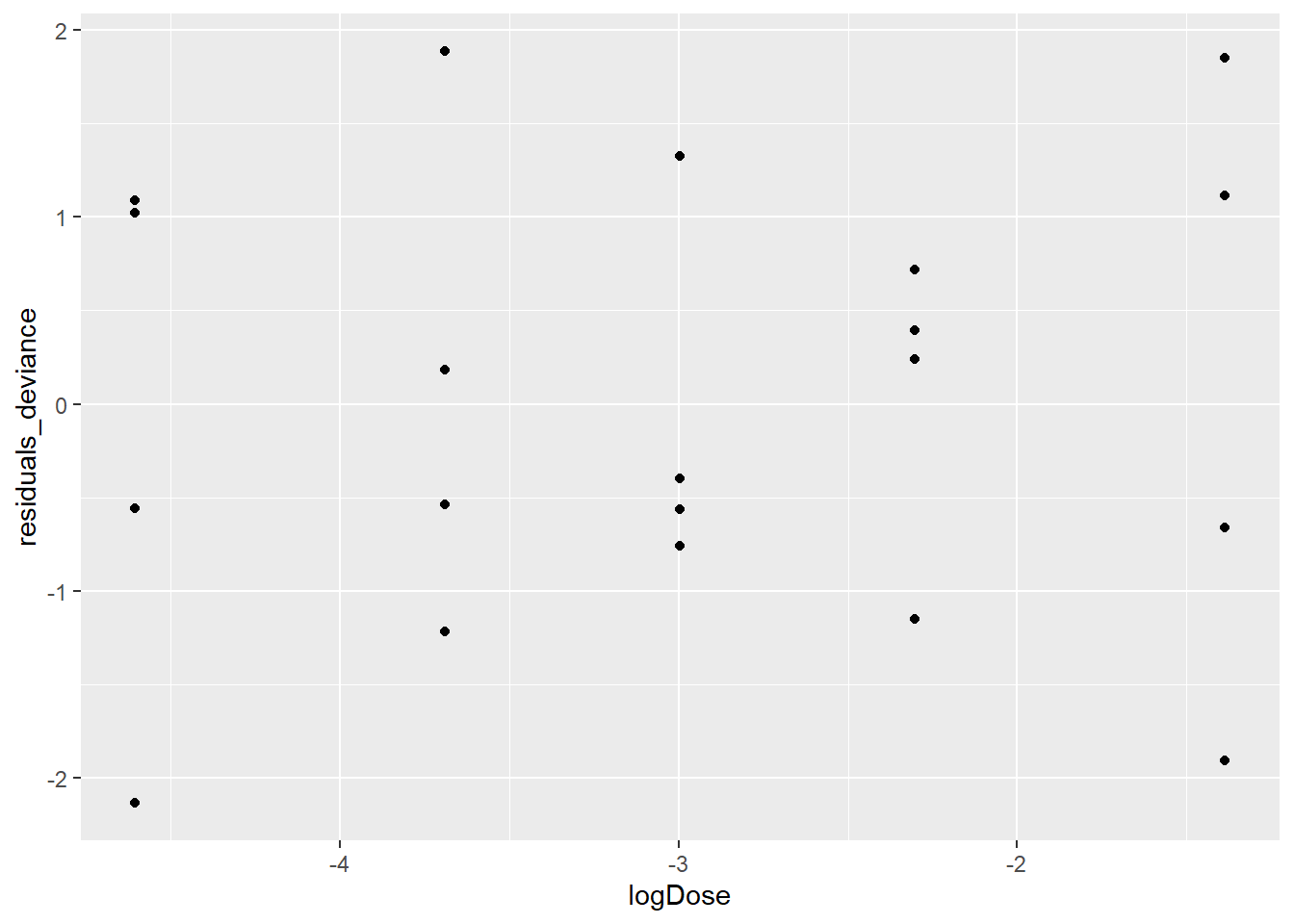

ggplot(data = tumors, aes(logDose,residuals_pearson)) + geom_point()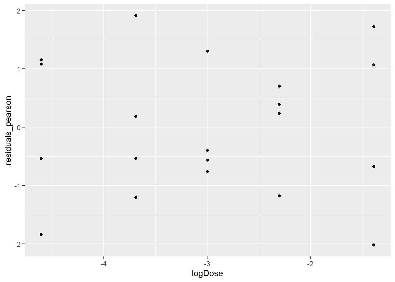

ggplot(data = tumors, aes(residuals_deviance,residuals_pearson)) + geom_point()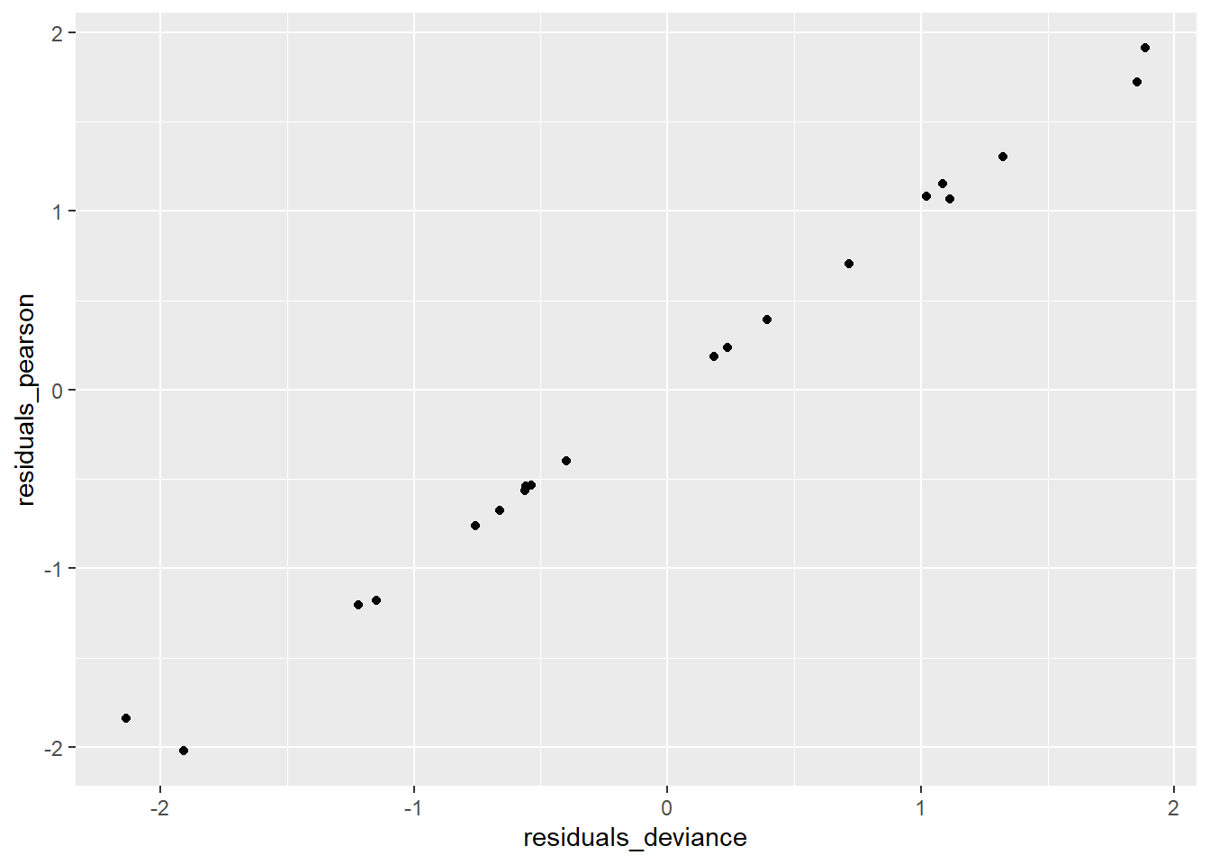

There are no obvious patterns in either of the plots showing the residuals against logDose, and there are also no outliers. This is all good, it suggests that we’ve done a good job at modeling the log odds of tumors (although we still have to talk about the over dispersion). We created the scatterplot of the Pearson residuals versus the deviance residuals just so you could see how similar they are. For the most part, they fall along the y = x diagonal.

When looking at residuals, it can also be useful to plot the residuals versus the fitted values of a model. Again, we’re hoping that we don’t see any patterns in such a plot:

tumors$fitted = predict.glm(mod7,scale="link")
ggplot(data = tumors, aes(fitted,residuals_deviance)) + geom_point()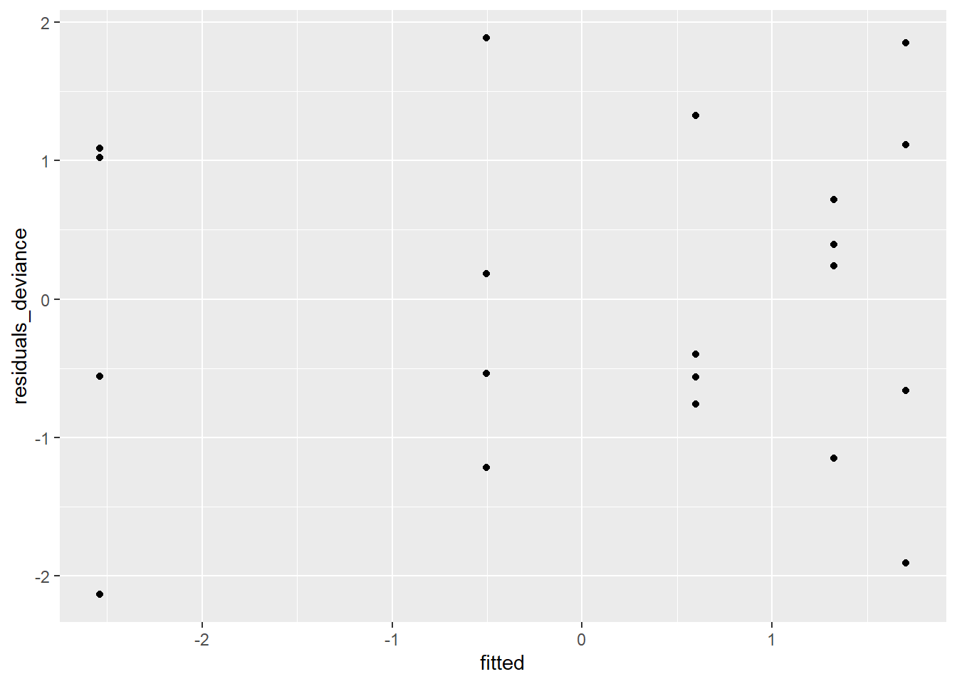

There are no clear patterns or problems with this plot, so again we have confirmation that we’re using a decent model at this point.

4 Dealing with over-dispersion

Over dispersion can arise when there is structure in the data that is not accounted for by a model. A high degree of over dispersion may indicate that important predictors have been omitted, the functional form of the predictors is inadequate to capture relevant features of the data, observations assumed independent are not so, or large outliers are present. When there is evidence of lack of fit, we expect overdispersion.

From the residuals of mod7 that we just examined (mod7 includes logDose + logDose2), it doesn’t seem that there are outliers. It also seems that we’ve gotten a good functional form for the predictors (i.e., logDose + logDose2). Is there even evidence of lack of fit here? We looked at the deviance goodness of fit above, but let’s repeat it here just for mod7:

LRstats(mod7)

	AIC	BIC	LR Chisq	Df	Pr(>Chisq)
mod7	119.4461	122.4333	26.04806	17	0.0735894

The p-value is 0.07, which suggests that our model is a good fit, but just barely. You also saw in the narrated lectures that the estimated dispersion parameter here is 1.48 not wildly larger than one, but larger nonetheless. Even though there may not be strong evidence for over dispersion here, it makes sense that the counts of fish with tumors are over dispersed because it’s not likely that measurements on fish from the same tank are statistically independent.

When in doubt, assume that counts are over dispersed.

You saw in the narrated lecture that the approach to use in the binomial setting when over dispersion is present is called quasi-binomial logistic regression. We’ll perform this in R, and then we’ll compare the model output from the quasi-binomial approach to the binomial approach in mod7.

mod8 <- glm(data = tumors, (Tumor/Total) ~ logDose + logDose2, weights = Total, family = "quasibinomial")
display(mod7)

glm(formula = (Tumor/Total) ~ logDose + logDose2, family = "binomial", 
    data = tumors, weights = Total)
            coef.est coef.se
(Intercept)  1.03     0.49  
logDose     -1.03     0.36  
logDose2    -0.39     0.06  
---
  n = 20, k = 3
  residual deviance = 26.0, null deviance = 667.2 (difference = 641.1)

display(mod8)

glm(formula = (Tumor/Total) ~ logDose + logDose2, family = "quasibinomial", 
    data = tumors, weights = Total)
            coef.est coef.se
(Intercept)  1.03     0.60  
logDose     -1.03     0.43  
logDose2    -0.39     0.07  
---
  n = 20, k = 3
  residual deviance = 26.0, null deviance = 667.2 (difference = 641.1)
  overdispersion parameter = 1.5

The fundamental change between mod7 and mod8 is that the standard errors of the regression coefficients in mod8, the quasi-binomial model are larger than they are in mod7. This illustrates the problem with ignoring a lack of statistical independence:

If responses are not statistically independent, but you fit a model that assumes statistical independence, the mistake you often make is that of underestimating standard errors. This results in p-values being smaller than they should be, and confidence intervals being more narrow than they should be.

A strong disadvantage of the quasi-likelihood (in this case quasi-binomial) approach is that since quasi-likelihoods are not real likelihoods, we cannot use likelihood-based methods of model comparison, like AIC and BIC, to choose between them, nor can we compare them with true likelihood models. Indeed, the idea of “model comparison” becomes somewhat muddled when we are talking about a collection of things that are not proper probability models to begin with.

You’ll learn about an alternative to the quasi-binomial model in Module 7 when we introduce mixed effects models. In that Module, we’ll refit the tumor data, including TankID as a random effect. You might wonder why we can’t just include TankID in our logistic regression model to address the over dispersion problem. Recall, however, that there are 20 tanks, so that if we use TankID in the model, we’ll gobble up all 20 data points before we can estimate all the “tank effects.” Look at what happens:

mod9 <- glm(data = tumors, (Tumor/Total) ~ logDose + logDose2 + TankID, weights = Total, family = "binomial")
summary(mod9)

Call:
glm(formula = (Tumor/Total) ~ logDose + logDose2 + TankID, family = "binomial", 
    data = tumors, weights = Total)

Coefficients: (2 not defined because of singularities)
            Estimate Std. Error z value Pr(>|z|)   
(Intercept)  0.33225    1.28208   0.259  0.79552   
logDose     -1.45660    1.00434  -1.450  0.14697   
logDose2    -0.43379    0.16314  -2.659  0.00784 **
TankID2     -0.62553    0.57989  -1.079  0.28073   
TankID3     -1.61328    0.79714  -2.024  0.04299 * 
TankID4      0.02598    0.49820   0.052  0.95842   
TankID5     -0.42670    0.39718  -1.074  0.28269   
TankID6      0.10437    0.39138   0.267  0.78973   
TankID7     -0.58424    0.40069  -1.458  0.14481   
TankID8     -0.26517    0.39306  -0.675  0.49991   
TankID9     -0.36920    0.40678  -0.908  0.36409   
TankID10    -0.32905    0.40933  -0.804  0.42147   
TankID11     0.09795    0.41529   0.236  0.81354   
TankID12    -0.29201    0.40849  -0.715  0.47471   
TankID13     0.04317    0.37730   0.114  0.90890   
TankID14     0.13158    0.38163   0.345  0.73027   
TankID15    -0.34740    0.35820  -0.970  0.33212   
TankID16          NA         NA      NA       NA   
TankID17    -0.32395    0.37597  -0.862  0.38888   
TankID18     0.85371    0.48207   1.771  0.07657 . 
TankID19     0.56157    0.44855   1.252  0.21058   
TankID20          NA         NA      NA       NA   
---
Signif. codes:  0 '***' 0.001 '**' 0.01 '*' 0.05 '.' 0.1 ' ' 1

(Dispersion parameter for binomial family taken to be 1)

    Null deviance: 6.6720e+02  on 19  degrees of freedom
Residual deviance: 6.2617e-14  on  0  degrees of freedom
AIC: 127.4

Number of Fisher Scoring iterations: 4

This model is over-saturated we’ve put too many terms in it, and not all of them can be estimated. Notice also that the degrees of freedom corresponding to the residual deviance is 0. We should not use this model for inference.

5 A Pitfall – perfect separation

In this section of the lab, we’ll discuss a pathology that can arise in logistic regression. We’ll show you what happens, and we’ll make a suggestion for dealing with the problem.

First, we’ll create some fake data:

y <- c(0,0,0,0,1,1,1,1)
x1 <-c(1,2,3,3,5,6,10,11)
x2 <-c(3,2,-1,-1,2,4,1,0)
df <- data.frame(y, x1, x2)
df

y	x1	x2
0	1	3
0	2	2
0	3	-1
0	3	-1
1	5	2
1	6	4
1	10	1
1	11	0

Take a look at a plot of the data below, and it will be easy to see what the potential problem is somewhere between 3 and 5, there’s perfect separation between the y = 0 responses and the y = 1 responses. The question is, where is “somewhere?”

ggplot(data = df, aes(x = x1, y = y)) +
 geom_point() +
 ggtitle("Note the clean split between 0's and 1's")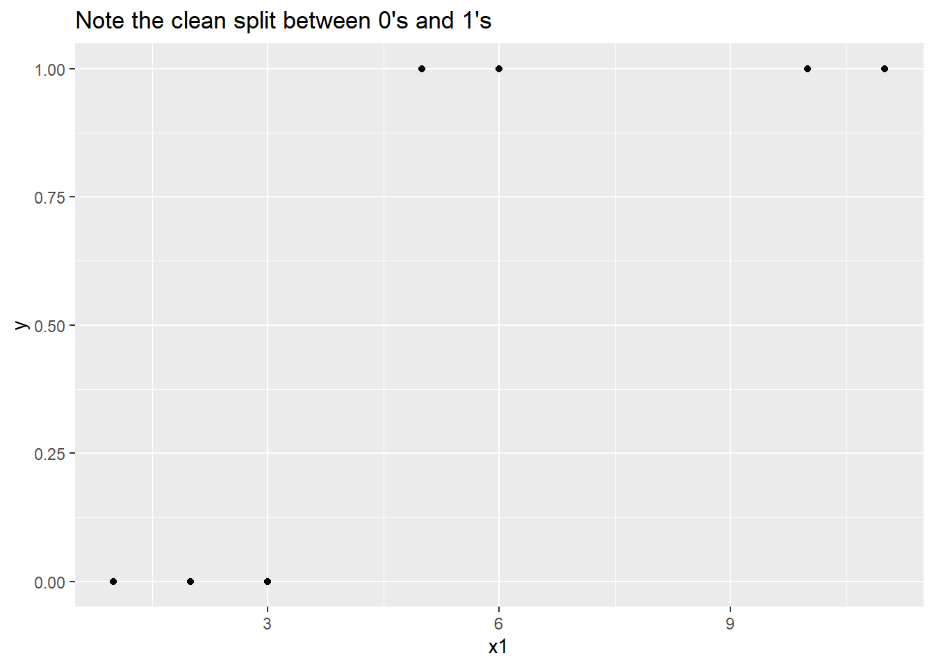

The following will not work try inserting an “r” to make it executable.

m1 <- glm(y ~ x1 + x2, family = binomial, data = df)

This generates an error, because x1 predicts too well. There is no unique “maximum likelihood estimate” for the coefficient on x1, because there are too many super-excellent solutions, and the numerical algorithm behind the glm() function just can’t choose. This might seem like the silliest possible problem to have that there are too many good solutions but saying that doesn’t make the algorithm converge.

If we really believe that we can predict y perfectly from x1, we could throw out the whole model and just write down a decision rule like “predict y = 1 if x1 >= 4, predict y = 0 otherwise.” Of course, we don’t know if this is a better or worse rule than, say, “predict y = 1 if x1 >= 3.5, predict y = 0 otherwise” the choice of ‘4’ as the cutpoint was arbitrary. That is, we might have the same problem that the glm() algorithm had, which cut-point is the best one?!

The real underlying issue here is that we should not believe that we’ve derived a perfect classifier (i.e., a decision rule that says when y = 1 and when y = 0) from 8 data points! In fact, in the fake data we created above, we also created a second explanatory variable, x2, and we never even used it.

An alternative approach sidesteps the problem by directly imposing our belief that a perfect classifier is too good to be true, and so it allows for estimating a coefficient on x1. This approach, a Bayesian generalized linear model, is well beyond the scope of this course, but you can nevertheless see it in action using the bayesglm() function in the arm package:

bayes1 <- bayesglm(y ~ x1 + x2, family = binomial, data = df, prior.df = 1)
summary(bayes1)

Call:
bayesglm(formula = y ~ x1 + x2, family = binomial, data = df, 
    prior.df = 1)

Coefficients:
            Estimate Std. Error z value Pr(>|z|)  
(Intercept)  -3.6937     1.9372  -1.907   0.0566 .
x1            0.7055     0.3863   1.826   0.0678 .
x2            0.3347     0.4448   0.752   0.4518  
---
Signif. codes:  0 '***' 0.001 '**' 0.01 '*' 0.05 '.' 0.1 ' ' 1

(Dispersion parameter for binomial family taken to be 1)

    Null deviance: 11.0904  on 7  degrees of freedom
Residual deviance:  2.4855  on 5  degrees of freedom
AIC: 8.4855

Number of Fisher Scoring iterations: 57

You should still take a careful look at this model summary. In particular there were 46 iterations of the Fisher scoring algorithm even with the prior specification about imperfect separation, the algorithm still took a while to find a solution.

6 Test for difference in proportions

Another important application of logistic regression is its use in testing the difference in two proportions. We’ll return to the Berkeley Admissions data to take a look.

 (UCBA_sum <- t(margin.table(UCBAdmissions,c(1,2))))

        Admit
Gender   Admitted Rejected
  Male       1198     1493
  Female      557     1278

And remember that we looked at the equivalence between prop.test() and chisq.test().

prop.test(UCBA_sum)

    2-sample test for equality of proportions with continuity correction

data:  UCBA_sum
X-squared = 91.61, df = 1, p-value < 2.2e-16
alternative hypothesis: two.sided
95 percent confidence interval:
 0.1129887 0.1703022
sample estimates:
   prop 1    prop 2 
0.4451877 0.3035422 

chisq.test(UCBA_sum)

    Pearson's Chi-squared test with Yates' continuity correction

data:  UCBA_sum
X-squared = 91.61, df = 1, p-value < 2.2e-16

Now let’s perform the same test, using logistic regression.

7 Check code: gender should be factor and admit is factor with 0 levels

UCBA_case <- expand.dft(UCBA_sum)
UCBA_case %<>% mutate(Gender=factor(Gender), Admit = relevel(factor(Admit),"Rejected"))
 #mutate(Admit = factor(Admit,levels(Admit)[2:1]))
 # make sure that "Rejected" is the failure level in glm
head(UCBA_case)

Gender	Admit
Male	Admitted
Male	Admitted
Male	Admitted
Male	Admitted
Male	Admitted
Male	Admitted

test1 <- glm(data = UCBA_case, Admit ~ Gender, family = binomial)
summary(test1)

Call:
glm(formula = Admit ~ Gender, family = binomial, data = UCBA_case)

Coefficients:
            Estimate Std. Error z value Pr(>|z|)    
(Intercept) -0.83049    0.05077 -16.357   <2e-16 ***
GenderMale   0.61035    0.06389   9.553   <2e-16 ***
---
Signif. codes:  0 '***' 0.001 '**' 0.01 '*' 0.05 '.' 0.1 ' ' 1

(Dispersion parameter for binomial family taken to be 1)

    Null deviance: 6044.3  on 4525  degrees of freedom
Residual deviance: 5950.9  on 4524  degrees of freedom
AIC: 5954.9

Number of Fisher Scoring iterations: 4

The relationship to prop.test() may not be immediately clear, and this is partly because the logistic regression output is on then model scale in this case the log odds. Take a look at the z value corresponding to the GenderMale variable. If you take the square of this value, you get 91.26, which is quite similar to the X squared value you get from prop.test() and from Chisq.test. Recall that the square of a standard Normal random variable is a Chi-square random variable, and this helps to explain the similarity.

If we perform the appropriate back-transformations from the logistic regression output, we’ll see the correspondence to the test for a difference in proportions:

plogis(-0.83049) #Pr(Admit|Female)

[1] 0.3035415

plogis(-0.83049+0.61035) # Pr(Admit|Male)

[1] 0.4451862

8 Lab 4 Assignment

Question

Here we will return to the UCBAdmissions dataset and fit a logistic regression model for the count of students admitted (out of the total applicants) for each combination of the factors gender and department.

Some tips for part (a):

• You can use the group argument to geom_line() to connect points within a group for instance, given a plot with Gender on the x axis and a variable called eLogits on the y, you could add geom_line(aes(group = Dept, x = Gender, y = eLogits)), where the slope of the connecting lines would correspond to the sign and magnitude of the difference in empirical logits (log of observed odds ratio) between genders within each department.

• You can also incorporate information about the total number of applicants to each department into your plot. For instance, supposing you had a data frame with separate columns containing counts of “Admitted” and “Rejected” by sex and department, you could map the number of applicants to the size of the plot points using geom_point(size = Admitted + Rejected).

a Plot

Fit a logistic regression model for the count of students admitted (out of the total applicants) for each combination of the factors gender and department.

1. Construct an informative ggplot() of the empirical logits of admission proportion vs gender and department. It’s up to you what aesthetics to map to which variables, there is more than one right answer here.

rm(list = ls())
data("UCBAdmissions")

df <- UCBAdmissions
df <- df |> as.data.frame()
df <- expand.dft(df)

admitted <- df |> filter(Admit == "Admitted") 
admitted <- admitted |> dplyr::select(-Admit)

b <- admitted |> group_by(Dept) |> dplyr::summarise(
  tot = n())

b <- left_join(admitted, b, by = "Dept")
a <- b |> group_by(Dept, Gender) |> reframe(
  tot = tot,
  counts = ifelse(Gender == "Female", 
                  sum(ifelse(Gender == "Female", 1, 0)), 
                  sum(ifelse(Gender == "Female", 0, 1)))
  )
a <- a |> unique()
a <- a |> mutate(elog = log((counts)/(tot-counts))
            )


a |> ggplot() + 
  aes(x = Gender, y = elog, color = Dept, group = Dept) + 
  geom_point(aes(size = as.factor(tot))) + 
  geom_line() + 
  labs(
    title = "Difference in the estimated log proportions admitted by gender and department", 
    subtitle = "The size of the points reflects the number of students admitted "
  )

Warning: Using size for a discrete variable is not advised.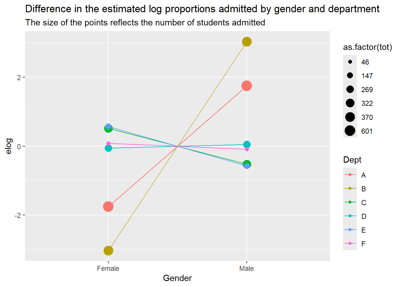

b <- df |> group_by(Dept, Admit, Gender) |> reframe(
  tot = n()) |> unique()

b <- b |> pivot_wider(names_from = "Admit", values_from = "tot")
c <- b |> group_by(Dept) |> reframe(tot_a = sum(Admitted), 
                               tot_r = sum(Rejected))
b <- left_join(b,c, by = "Dept") |> 
  mutate(tot = tot_a + tot_r, 
         tot_f = Admitted + Rejected
         )
b |> head()

Dept	Gender	Admitted	Rejected	tot_a	tot_r	tot	tot_f
A	Female	89	19	601	332	933	108
A	Male	512	313	601	332	933	825
B	Female	17	8	370	215	585	25
B	Male	353	207	370	215	585	560
C	Female	202	391	322	596	918	593
C	Male	120	205	322	596	918	325

a <- b |> mutate(
  elog_a = log((Admitted)/(tot_a)),
  elog_r = log((Rejected)/(tot_r))
            )


a |> ggplot() + 
  aes(x = Gender, y = elog_a, color = Dept, group = Dept) + 
  geom_point(aes(size = as.factor(tot_f))) + 
  geom_line() + 
  labs(
    title = "Difference in the estimated log proportions admitted by gender and department", 
    subtitle = "The size of the points reflects the number of students who applied"
  ) +
  guides(size = "none")

Warning: Using size for a discrete variable is not advised.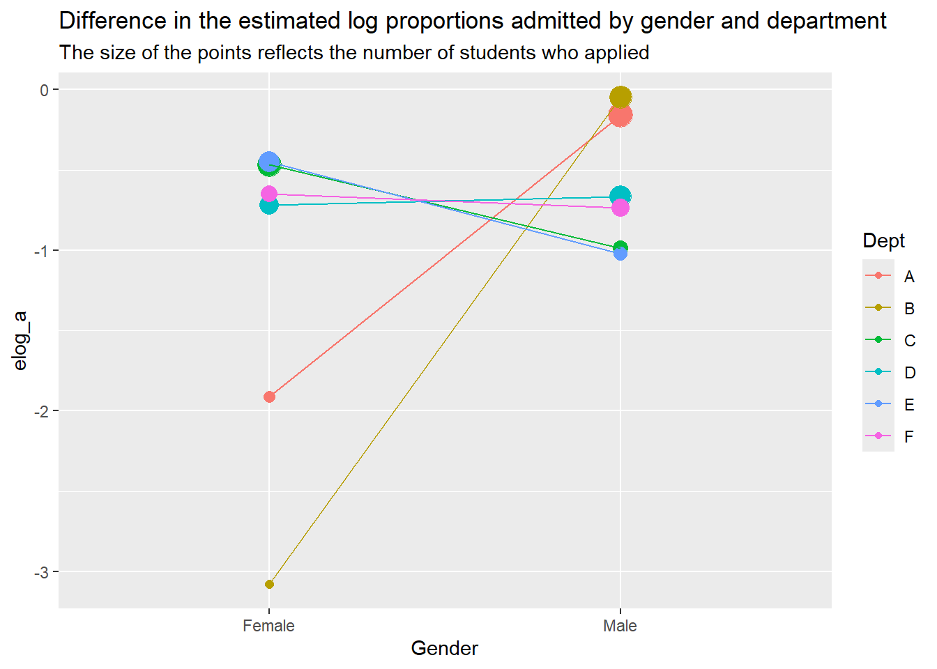

b variability in admissions

2. Based on your plot from (a), which variable (gender or department) appears to account for more of the variability in admissions? Explain.

It looks like regardless of department, the number of people admitted depends more on the number of applicants than it does on gender. Different departments seem to have a larger gender disparity. Departments A and B account for most of the variability.

c Fit

3. Fit an appropriate (binomial) logistic regression model for admissions. What is the estimated dispersion parameter? Is there evidence of lack of fit?

Fitting a logistic regression model for the count of students admitted (out of the total applicants) for each combination of the factors gender and department.

c <- a |> dplyr::select(Dept, Gender, admit = Admitted, rej = Rejected, tot = tot_f, tot_a, elog_a, elog_r)
# str(c)
c <- c |> mutate(Dept = factor(Dept), 
                 Gender = factor(Gender))
c |> head()

Dept	Gender	admit	rej	tot	tot_a	elog_a	elog_r
A	Female	89	19	108	601	-1.9099586	-2.8606960
A	Male	512	313	825	601	-0.1602703	-0.0589318
B	Female	17	8	25	370	-3.0802897	-3.2911965
B	Male	353	207	560	370	-0.0470349	-0.0379192
C	Female	202	391	593	322	-0.4662838	-0.4215331
C	Male	120	205	325	322	-0.9870598	-1.0672307

m1 <- glm(
  data = c, 
  family = "binomial",
  cbind(admit, rej) ~ Gender + Dept)
summary(m1)

Call:
glm(formula = cbind(admit, rej) ~ Gender + Dept, family = "binomial", 
    data = c)

Coefficients:
            Estimate Std. Error z value Pr(>|z|)    
(Intercept)  0.68192    0.09911   6.880 5.97e-12 ***
GenderMale  -0.09987    0.08085  -1.235    0.217    
DeptB       -0.04340    0.10984  -0.395    0.693    
DeptC       -1.26260    0.10663 -11.841  < 2e-16 ***
DeptD       -1.29461    0.10582 -12.234  < 2e-16 ***
DeptE       -1.73931    0.12611 -13.792  < 2e-16 ***
DeptF       -3.30648    0.16998 -19.452  < 2e-16 ***
---
Signif. codes:  0 '***' 0.001 '**' 0.01 '*' 0.05 '.' 0.1 ' ' 1

(Dispersion parameter for binomial family taken to be 1)

    Null deviance: 877.056  on 11  degrees of freedom
Residual deviance:  20.204  on  5  degrees of freedom
AIC: 103.14

Number of Fisher Scoring iterations: 4

\(\hat{\psi} = 20.204/5 =\)

20.204/5

[1] 4.0408

There appears to be considerable dispersion

pchisq(20.204, 5, lower.tail = F)

[1] 0.001144215

There is evidence of lack of fit. The p-value is low.

d plot of residuals vs fitted values

4. Construct a plot of residuals vs fitted values (try just plot-ing your fitted model object). From this plot, can you identify a source for any fit problems encountered in part (c)?

c$fitted <- predict.glm(m1, scale = "link")
c$resids_d <- residuals(m1)
c$resids_p <- residuals(m1, type = "pearson")
ggplot(c) + 
  aes(tot_a, resids_d) + 
  geom_point()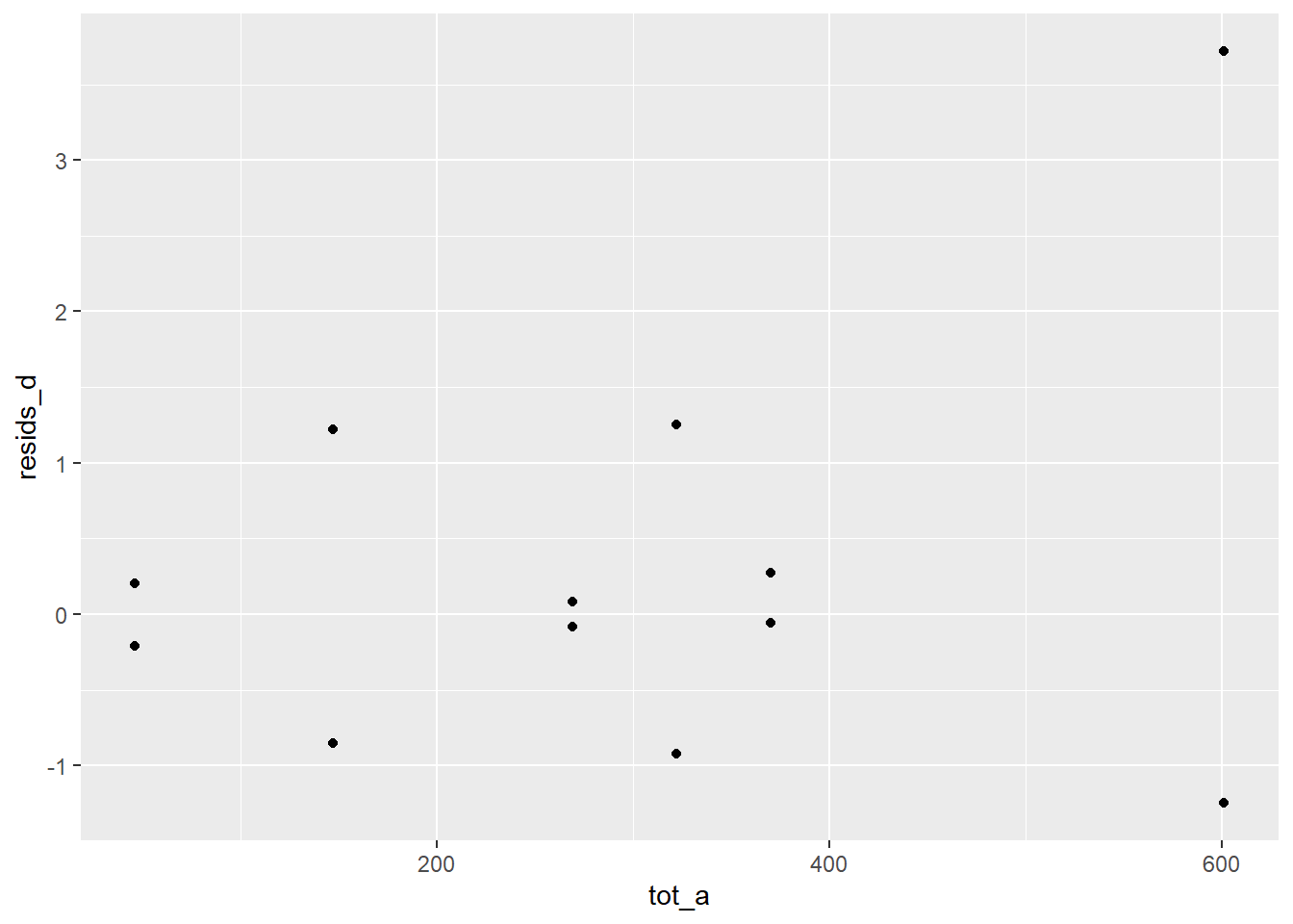

ggplot(c) + 
  aes(tot_a, resids_p) + 
  geom_point()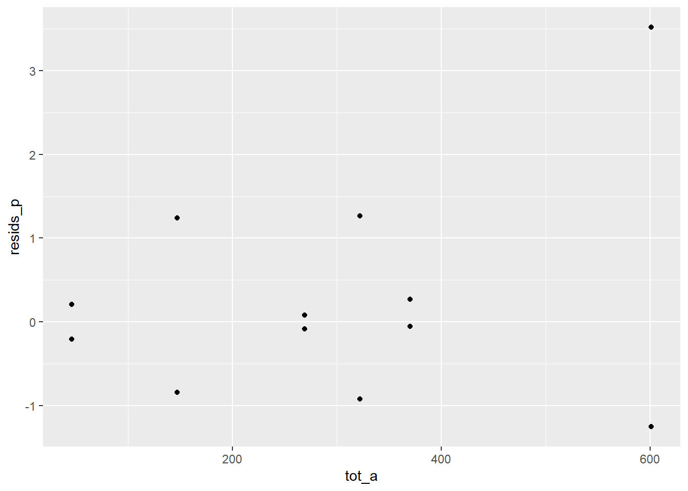

ggplot(c) + 
  aes(fitted, resids_d) + 
  geom_point(aes(color = Dept, size = Gender))

Warning: Using size for a discrete variable is not advised.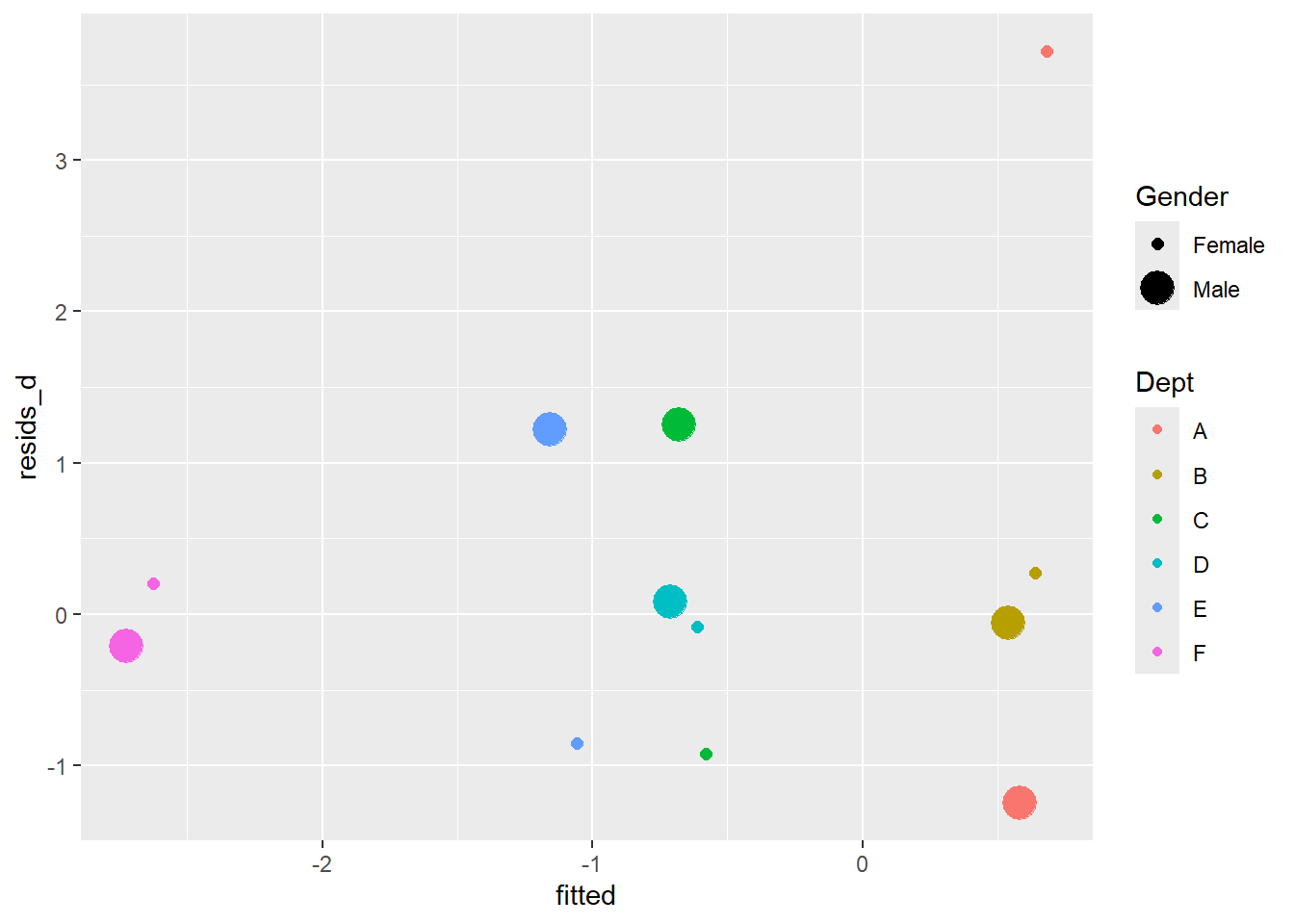

There is an outlier in Department A females. The other departments accepted roughly equal proportions by gender, but dept A accepted about 20% more for female applicants.

c |> mutate(prop = admit/tot) |> relocate(prop, .after = tot) |> head()

Dept	Gender	admit	rej	tot	prop	tot_a	elog_a	elog_r	fitted	resids_d	resids_p
A	Female	89	19	108	0.8240741	601	-1.9099586	-2.8606960	0.6819215	3.7189203	3.5186674
A	Male	512	313	825	0.6206061	601	-0.1602703	-0.0589318	0.5820514	-1.2486740	-1.2538077
B	Female	17	8	25	0.6800000	370	-3.0802897	-3.2911965	0.6385236	0.2706080	0.2689516
B	Male	353	207	560	0.6303571	370	-0.0470349	-0.0379192	0.5386535	-0.0560085	-0.0560205
C	Female	202	391	593	0.3406408	322	-0.4662838	-0.4215331	-0.5806765	-0.9243398	-0.9207783
C	Male	120	205	325	0.3692308	322	-0.9870598	-1.0672307	-0.6805466	1.2533375	1.2628723

d2 Refit

4. Refit the binomial model above, but excluding the data from department A. Now what is the estimated dispersion parameter? Based on the p-value, what would you conclude about the effect of Gender on admissions (to departments other than A) using this model?

d <- c |> filter(Dept != "A")

# m1 <- glm(
#   data = c, 
#   family = "binomial",
#   cbind(admit, rej) ~ Gender + Dept)
# summary(m1)

m2 <- glm(cbind(admit, rej) ~ Gender + Dept, 
          family = "binomial", 
          data = d)
summary(m2)

Call:
glm(formula = cbind(admit, rej) ~ Gender + Dept, family = "binomial", 
    data = d)

Coefficients:
            Estimate Std. Error z value Pr(>|z|)    
(Intercept)  0.51349    0.11936   4.302 1.69e-05 ***
GenderMale   0.03069    0.08676   0.354    0.724    
DeptC       -1.14008    0.12188  -9.354  < 2e-16 ***
DeptD       -1.19456    0.11984  -9.968  < 2e-16 ***
DeptE       -1.61308    0.13928 -11.581  < 2e-16 ***
DeptF       -3.20527    0.17880 -17.927  < 2e-16 ***
---
Signif. codes:  0 '***' 0.001 '**' 0.01 '*' 0.05 '.' 0.1 ' ' 1

(Dispersion parameter for binomial family taken to be 1)

    Null deviance: 539.4581  on 9  degrees of freedom
Residual deviance:   2.5564  on 4  degrees of freedom
AIC: 71.791

Number of Fisher Scoring iterations: 3

Now what is the estimated dispersion parameter? Based on the p-value, what would you conclude about the effect of Gender on admissions (to departments other than A) using this model?

\(\hat{\psi} = 2.5564/4 =\)

2.5564/4

[1] 0.6391

There is now no extra binomial variation

# 2.5564  on 4
pchisq(2.5564, 4, lower.tail = F)

[1] 0.6345658

There is no evidence of lack of fit. It appears there is no evidence of discrimination on the basis of gender outside of department A.

e Confint

5. The approach in part (d) allowed us to keep the binomial likelihood model, but only by performing an unprincipled exclusion of some apparently-legitimate data that happened to be “outlying”.

To avoid this, we’ll refit the model for all departments with the quasibinomial family.

Using the quasibinomial model for all departments, what do you conclude about the effect of Gender on admissions? Support your conclusion by constructing and interpreting a 95% confidence interval for

\(P_{diff} = [P(Admit | (Department, Male)) - P(Admit | (Department, Female))]\)

That is, construct an interval on the model scale, then back-transform to the data scale. Be careful with the direction (male higher or female higher) of the observed difference in conditional probability of admission.

1. fit a quasibinomial
2. conclusion for gender on admissions.
3. construct CI for difference in probability m - f, and interpret

• consruct on model scale
• back-transform to data scale
• care for direction

1. fit a quasibinomial

c <- c |> dplyr::select(dept = Dept, gender = Gender, admit, rej, tot, tot_a, elog_a, elog_r)
c <- c |> mutate(prop = admit/tot) |> relocate(prop, .after = tot)

# m1 <- glm(
#   data = c, 
#   family = "binomial",
#   cbind(admit, rej) ~ Gender + Dept)

m3 <- glm(data = c, 
          family = "quasibinomial", 
          cbind(admit, rej) ~ gender + dept)
s3 <- summary(m3)
s3

Call:
glm(formula = cbind(admit, rej) ~ gender + dept, family = "quasibinomial", 
    data = c)

Coefficients:
            Estimate Std. Error t value Pr(>|t|)    
(Intercept)  0.68192    0.19231   3.546 0.016458 *  
genderMale  -0.09987    0.15687  -0.637 0.552355    
deptB       -0.04340    0.21312  -0.204 0.846672    
deptC       -1.26260    0.20690  -6.102 0.001711 ** 
deptD       -1.29461    0.20533  -6.305 0.001477 ** 
deptE       -1.73931    0.24470  -7.108 0.000854 ***
deptF       -3.30648    0.32982 -10.025 0.000169 ***
---
Signif. codes:  0 '***' 0.001 '**' 0.01 '*' 0.05 '.' 0.1 ' ' 1

(Dispersion parameter for quasibinomial family taken to be 3.764856)

    Null deviance: 877.056  on 11  degrees of freedom
Residual deviance:  20.204  on  5  degrees of freedom
AIC: NA

Number of Fisher Scoring iterations: 4

logistic <- function(x){exp(x)/(1 + exp(x))}
odds <- exp(m3$coefficients)
prob <- logistic(m3$coefficients)
odds

(Intercept)  genderMale       deptB       deptC       deptD       deptE 
 1.97767415  0.90495497  0.95753028  0.28291804  0.27400567  0.17564230 
      deptF 
 0.03664494 

# prob
# plogis(m3$coefficients)

2. conclusion for gender on admissions.

Using the quasibinomial model for all departments, what do you conclude about the effect of Gender on admissions?

logodds_admit <- function(f=0,m=0, B=0,C=0,D=0,E=0,F_=0) {
  (0.68192148*f) + ((0.68192148 - 0.09987009)*m) + 
  (-0.04339793*B) + (-1.26259802*C) + 
  (-1.29460647*D) + (-1.73930574*E) + 
  (-3.30648006*F_)
}

female <- c(
logodds_admit(f= 1),
logodds_admit(f=1, B= 1),
logodds_admit(f=1, C= 1),
logodds_admit(f=1, D= 1),
logodds_admit(f=1, E= 1),
logodds_admit(f=1, F_=1))

male <- c(
logodds_admit(m=1),
logodds_admit(m=1, B= 1),
logodds_admit(m=1, C= 1),
logodds_admit(m=1, D= 1),
logodds_admit(m=1, E= 1),
logodds_admit(m=1, F_= 1))

f_odds <- female |> exp()
m_odds <- male|> exp()
# f_odds
# m_odds

round(plogis(female)*100, 2)

[1] 66.42 65.44 35.88 35.14 25.78  6.76

round(plogis(male)*100, 2)

[1] 64.15 63.15 33.61 32.90 23.92  6.15

The probability of males or females making it into any given departments are estimated to be roughly equal.

3. construct CI

3. construct CI for difference in probability m - f, and interpret

• consruct on model scale
• back-transform to data scale
• care for direction

Support your conclusion by constructing and interpreting a 95% confidence interval for

\(P_{diff} = [P(Admit | (Department, Male)) - P(Admit | (Department, Female))]\)

ci3 <- confint.default(m3)
ci3

                 2.5 %     97.5 %
(Intercept)  0.3049994  1.0588436
genderMale  -0.4073263  0.2075862
deptB       -0.4611114  0.3743155
deptC       -1.6681191 -0.8570769
deptD       -1.6970492 -0.8921637
deptE       -2.2189109 -1.2597006
deptF       -3.9529149 -2.6600453

# ci3 |> exp()
# (ci3 |> exp())^-1

ci3[2] |> exp()

[1] 0.665427

ci3[9] |> exp()

[1] 1.230704

0.665427^-1

[1] 1.502794

1.230704

[1] 1.230704

The ratio of students admitted by sex is estimated to be 1.11 females per male. With 95% confidence, the upper and lower bounds of the ratio of admitted students is between 1.5 females per male and 1.23 males per female. Department doesn’t matter.

coefs <- m3$coefficients
coefs

(Intercept)  genderMale       deptB       deptC       deptD       deptE 
 0.68192148 -0.09987009 -0.04339793 -1.26259802 -1.29460647 -1.73930574 
      deptF 
-3.30648006 

0.68192148 -0.09987009

[1] 0.5820514

exp(-0.09987009)^-1

[1] 1.105027

1.35662419*0.66542700 

[1] 0.9027344

2.88303501*1.23070375

[1] 3.548162

2.038727/(2.038727+1)

[1] 0.6709148

logodds_admit <- function(f=0,m=0, B=0,C=0,D=0,E=0,F_=0) {
  (0.68192148*f) + ((0.68192148 - 0.09987009)*m) + 
  (-0.04339793*B) + (-1.26259802*C) + 
  (-1.29460647*D) + (-1.73930574*E) + 
  (-3.30648006*F_)
}

female <- c(
logodds_admit(f= 1),
logodds_admit(f=1, B= 1),
logodds_admit(f=1, C= 1),
logodds_admit(f=1, D= 1),
logodds_admit(f=1, E= 1),
logodds_admit(f=1, F_=1))

male <- c(
logodds_admit(m=1),
logodds_admit(m=1, B= 1),
logodds_admit(m=1, C= 1),
logodds_admit(m=1, D= 1),
logodds_admit(m=1, E= 1),
logodds_admit(m=1, F_= 1))

f_odds <- female |> exp()
m_odds <- male|> exp()
# f_odds
# m_odds

round(plogis(female)*100, 2)

[1] 66.42 65.44 35.88 35.14 25.78  6.76

round(plogis(male)*100, 2)

[1] 64.15 63.15 33.61 32.90 23.92  6.15

coefs <- m3$coefficients
coefs

(Intercept)  genderMale       deptB       deptC       deptD       deptE 
 0.68192148 -0.09987009 -0.04339793 -1.26259802 -1.29460647 -1.73930574 
      deptF 
-3.30648006 

est <- s3$coefficients[1:7]
est

[1]  0.68192148 -0.09987009 -0.04339793 -1.26259802 -1.29460647 -1.73930574
[7] -3.30648006

SE <- s3$coefficients[8:14]
SE

[1] 0.1923107 0.1568683 0.2131230 0.2069023 0.2053317 0.2447010 0.3298197

ci3 <- confint.default(m3)
ci3

                 2.5 %     97.5 %
(Intercept)  0.3049994  1.0588436
genderMale  -0.4073263  0.2075862
deptB       -0.4611114  0.3743155
deptC       -1.6681191 -0.8570769
deptD       -1.6970492 -0.8921637
deptE       -2.2189109 -1.2597006
deptF       -3.9529149 -2.6600453

coefs[1]

(Intercept) 
  0.6819215 

SE[1]

[1] 0.1923107

coefs[1] + SE[1]*qnorm(.975)

(Intercept) 
   1.058844 

coefs[1] - SE[1]*qnorm(.975)

(Intercept) 
  0.3049994 

test <- data.frame(group = c("fa","ma", 'fb', 'fc', 'fd', 'fe', 'ff'),
                   est = est, 
                   se = SE, 
                   crt_v = rep(qnorm(.975), 7))

test <- test |> mutate(low = est - se*crt_v,
                       upp = est + se*crt_v)

# test2 |> dplyr::select(gro)

female

[1]  0.6819215  0.6385235 -0.5806765 -0.6126850 -1.0573843 -2.6245586

ci3

                 2.5 %     97.5 %
(Intercept)  0.3049994  1.0588436
genderMale  -0.4073263  0.2075862
deptB       -0.4611114  0.3743155
deptC       -1.6681191 -0.8570769
deptD       -1.6970492 -0.8921637
deptE       -2.2189109 -1.2597006
deptF       -3.9529149 -2.6600453

female

[1]  0.6819215  0.6385235 -0.5806765 -0.6126850 -1.0573843 -2.6245586

male

[1]  0.5820514  0.5386535 -0.6805466 -0.7125551 -1.1572544 -2.7244287

round(plogis(female)*100, 2)

[1] 66.42 65.44 35.88 35.14 25.78  6.76

round(plogis(male)*100, 2)

[1] 64.15 63.15 33.61 32.90 23.92  6.15

Diff in prob m - f

coefs

(Intercept)  genderMale       deptB       deptC       deptD       deptE 
 0.68192148 -0.09987009 -0.04339793 -1.26259802 -1.29460647 -1.73930574 
      deptF 
-3.30648006 

f <- c()
f <- append(f, logodds_admit(f=1))
f <- append(f, logodds_admit(f=1, B = 1))
f <- append(f, logodds_admit(f=1, C = 1))
f <- append(f, logodds_admit(f=1, D = 1))
f <- append(f, logodds_admit(f=1, E = 1))
f <- append(f, logodds_admit(f=1, F_= 1))

m <- c()
m <- append(m, logodds_admit(m=1))
m <- append(m, logodds_admit(m=1, B = 1))
m <- append(m, logodds_admit(m=1, C = 1))
m <- append(m, logodds_admit(m=1, D = 1))
m <- append(m, logodds_admit(m=1, E = 1))
m <- append(m, logodds_admit(m=1, F_= 1))

f

[1]  0.6819215  0.6385235 -0.5806765 -0.6126850 -1.0573843 -2.6245586

m

[1]  0.5820514  0.5386535 -0.6805466 -0.7125551 -1.1572544 -2.7244287

exp(m)

[1] 1.78970605 1.71369775 0.50634014 0.49038961 0.31434809 0.06558366

exp(0.58205)

[1] 1.789704

plogis(male) 

[1] 0.64153929 0.63149912 0.33613931 0.32903451 0.23916654 0.06154717

plogis(female)

[1] 0.6641674 0.6544196 0.3587769 0.3514470 0.2578096 0.0675745

# Pr(Admit|Male) - Pr(Admit|Female)
(plogis(male) - plogis(female))*100

[1] -2.2628122 -2.2920508 -2.2637625 -2.2412452 -1.8643101 -0.6027326

Females are estimated to be favored by about 2% in all departments except F. There they are only favored by about 0.6%

female |> exp()

[1] 1.97767415 1.89368289 0.55951970 0.54189393 0.34736323 0.07247174

male |> exp()

[1] 1.78970605 1.71369775 0.50634014 0.49038961 0.31434809 0.06558366

exp(-0.09987009)

[1] 0.904955

1.97767415 *0.904955

[1] 1.789706

1.89368289 *0.904955

[1] 1.713698

Scratch

That is, construct an interval on the model scale, then back-transform to the data scale. Be careful with the direction (male higher or female higher) of the observed difference in conditional probability of admission.

0.68192 + qt(p = .975, df = 11) * 0.19231 

[1] 1.105191

0.68192 - qt(p = .975, df = 11) * 0.19231 

[1] 0.2586485

Why don’t these match?

ci <- confint.default(m3)
ci

                 2.5 %     97.5 %
(Intercept)  0.3049994  1.0588436
genderMale  -0.4073263  0.2075862
deptB       -0.4611114  0.3743155
deptC       -1.6681191 -0.8570769
deptD       -1.6970492 -0.8921637
deptE       -2.2189109 -1.2597006
deptF       -3.9529149 -2.6600453

-0.09987 0.15687

exp(ci)

                 2.5 %     97.5 %
(Intercept) 1.35662419 2.88303501
genderMale  0.66542700 1.23070375
deptB       0.63058244 1.45399583
deptC       0.18860147 0.42440082
deptD       0.18322338 0.40976816
deptE       0.10872746 0.28373897
deptF       0.01919866 0.06994506

j <- m3$coefficients
j

(Intercept)  genderMale       deptB       deptC       deptD       deptE 
 0.68192148 -0.09987009 -0.04339793 -1.26259802 -1.29460647 -1.73930574 
      deptF 
-3.30648006 

m3$coefficients[3]

      deptB 
-0.04339793 

Probs

\(P_{diff} = [P(Admit | (Department, Male)) - P(Admit | (Department, Female))]\)

# male v female department a
# plogis(0.68192) # P(a|f,a)
plogis(j[1]) # P(a|f,a)

(Intercept) 
  0.6641674 

# plogis(0.68192-0.09987)# P(a|m,a)
plogis(j[1] + j[2])

(Intercept) 
  0.6415393 

The difference for all sets below favor the females.

plogis(j[1] + j[2]) - plogis(j[1])

(Intercept) 
-0.02262812 

In department a female has slightly higher probability of admittance.

# m v f, dept b
plogis(j[2] + j[3]) - plogis(j[1] + j[3])

genderMale 
-0.1901755 

In department B, female has more probability of admittance.

# # m v f, dept c
plogis(j[2] + j[4])- plogis(j[1] + j[4])

genderMale 
-0.1549375 

Again, female is more probale.

# # m v f, dept d
plogis(j[2] + j[5])- plogis(j[1] + j[5])# P(a|f,d)

genderMale 
-0.1527529 

# # m v f, dept e
plogis(j[2] + j[6])- plogis(j[1] + j[6])# P(a|f,e)

genderMale 
-0.1206608 

# # m v f, dept e
plogis(j[2] + j[7])- plogis(j[1] + j[7])# P(a|f,f)

genderMale 
-0.0354769 

ci3 |> exp()

                 2.5 %     97.5 %
(Intercept) 1.35662419 2.88303501
genderMale  0.66542700 1.23070375
deptB       0.63058244 1.45399583
deptC       0.18860147 0.42440082
deptD       0.18322338 0.40976816
deptE       0.10872746 0.28373897
deptF       0.01919866 0.06994506