library(tidyverse)3 Log Reg I
Learning Objectives
After successful completion of this module, you will be able to:
- Describe the logistic regression model, which includes a probability model for the responses and the model equation.
- Write a few sentences in non-technical language that explain the results of a logistic regression model fit.
- Describe how to compare two logistic regression models.
- Explain the need for the link function in logistic regression.
In R:
- Fit logistic regression models and interpret the output.
- Create exploratory plots for logistic regression, and be able to explain any limitations of these plots.
- Prepare and submit an R markdown script.
Task list
In order to achieve these learning outcomes, please make sure to complete the following:
- Review Module 3 Readings and
LecturesSubmit Module 3 HomeworkSubmit Module 3 LabTake the Module 3 Content QuizR QuizParticipate in the Module 3 Discussion
95% Confidence Interval for a standard normal distribution.
\[ CONF.INT = EST \pm SE*1.96 \]
Otherwise
\[ CONF.INT = EST \pm t_{\alpha = .05}\times SE \]
\[ Critcal \ Value = t_{\alpha = .05} \] \[ SE = \frac{sd}{sqrt(n)} \]
Donner.R, Lecture 4 Fitting Models.
Code
#
# R code to create a plot of the Donner party data and fit
# a logistic regression model
#

# install.packages("Sleuth3)

library(Sleuth3)
library(ggplot2)

#
# I like to create a "work" file for the current data file that
# I'm using; then I take a quick look at the data and create the
# Female indicator variable:
#

work = case2001
head(work)| Age | Sex | Status |
|---|---|---|
| 23 | Male | Died |
| 40 | Female | Survived |
| 40 | Male | Survived |
| 30 | Male | Died |
| 28 | Male | Died |
| 40 | Male | Died |
Code
work$Female = ifelse(work$Sex=="Female",1,0)

#
# Now, just a quick plot to look at the data (you'll do this
# in this module's lab too)
#

ggplot(work,aes(Age,Status,color=Sex)) + geom_point()
Code
#
# Here's the code to fit a logistic regression model:
#

LRM = glm(Status~Age+Female,data=work,family=binomial(link="logit"))
# summary(LRM)

#
# And approximate confidence intervals for the Beta's:
#

cis = confint.default(LRM)
# cis
# exp(cis)
W-3 Lectures
Introduction to Logistic Regression
Donner party survival by sex and age, interested in sex.
MLR won’t work, Binary responses are not Normally Distributed.
MLR was y = B + B1X1 + …
In Log-Reg:
g(u) = B + B1X1 + …
g(u) is the link function. Some function of the mean of y given the explanatory variables. For normally distributed responses, the link fct is the identity function.
For binary responses we use the logit link, g(p) = log(p/(1-p)). The log(odds) of success.
We’ll be able to interpret regression coefficient estimates from a logistic regression as changes in the odds of success corresponding to unit increases in an explanatory variable, with other variables held fixed. Or we can transform it back with:
\(p = f(\eta) = \frac{e^{\eta}}{1 + e^{\eta}}\)
eta is the greek letter
The Logistic regression model is:
\(logit(p) = \beta_0 + \beta_1X_1 + ...\)
It is classed as a general linear model with MLR.
Model Interpretation
Logit is log odd, if we exp(logit) we get odds.
\(\frac{p}{1-p} = exp(\beta_0 + \beta_1X_1 + ...)\)
\(\hat{logit (p)} = 1.63−0.078Age +1.60Female\)
LRM = glm(Status~Age+Female,data=work,family=binomial(link="logit"))
summary(LRM)
Call:
glm(formula = Status ~ Age + Female, family = binomial(link = "logit"),
    data = work)

Coefficients:
            Estimate Std. Error z value Pr(>|z|)
(Intercept)  1.63312    1.11018   1.471   0.1413
Age         -0.07820    0.03728  -2.097   0.0359 *
Female       1.59729    0.75547   2.114   0.0345 *
---
Signif. codes:  0 '***' 0.001 '**' 0.01 '*' 0.05 '.' 0.1 ' ' 1

(Dispersion parameter for binomial family taken to be 1)

    Null deviance: 61.827  on 44  degrees of freedom
Residual deviance: 51.256  on 42  degrees of freedom
AIC: 57.256

Number of Fisher Scoring iterations: 4
From the equation above we can get odds by specifying values for age and sex.
- The estimated odds of survival for a 50 year old female were: \(exp(1.63−0.078×50+1.60) = 0.52\)
- the odds of survival for a 50 year old male were: \(exp(1.63−0.078×50) = 0.10\)
The odds for a women were 5 times that of men.
The coefficient for age of men and women is the same in the equation/model, so odds are the same for all ages.
Estimation in Logistic Regression
Maximum Likelihood Estimation
The Bernoulli Likelihood
MLE in Logistic Regression
Inference
For MLR we use least squares for estimating coefficients.
For LogIts we use Maximum Likelihood Estimation
After specifying a statistical model for the response, we can write a Liklihood fct.
Some probability models for response variables—the Normal distribution, the Bernoulli distribution, the Binomial distribution, etc.
For each of these distributions, and given a sample of data, we can then construct a Likelihood function.
The maximum likelihood estimate (MLE), is the estimated value of our parameter(s) that maximize(s) the Likelihood function.
\prod_{i=1}^{\infty} a_{i}\(\prod_{i=1}^{\infty} a_{i}\)
For n independent Bernoulli (binary) random variables, each with it’s own prob of success p_i:
\(P(Y_i = y_i) = p_i^{y_i}(1-p_i)^{1-y_i}\)
The joint probability distribution of Y 1 to n is called the Likelihood Fucntion. It is the product of these n Bernoulli prob dists:
\(L(Y) = (Y_1 = y_1, Y_2 = y_2 + ...) = \prod_{i=1}^{n} p_i^{y_i}(1-p_i)^{1-y_i}\)
\(p_1^{y_1}(1-p_1)^{1-y_1} \times p_2^{y_2}(1-p_2)^{1-y_2} \times ...\)
for each pi, we’ll use its connection to the explanatory information using the logistic regression model.
The Bernoulli Likelihood Funtion.
\(L(Y) = \prod_{i=1}^{n} p_i^{y_i}(1-p_i)^{1-y_i}\)
where p_i is:
\(pi = \frac{exp(\beta_0 +\beta_1Age_i +\beta_2Female_i)}{1+exp(\beta_0 +\beta_1Age_i +\beta_2Female_i)}\)
So we sub in the expression for p_i into g(u):
\[ L(Y) = \prod_{i=1}^{n} ( \frac{exp(\beta_0 +\beta_1Age_i +\beta_2Female_i)}{1+exp(\beta_0 +\beta_1Age_i +\beta_2Female_i)} )^{y_i}( \frac{1}{1+exp(\beta_0 +\beta_1Age_i +\beta_2Female_i)} )^{1-y_i} \] This is the expression for the Bernoulli likelihood of the betas.
The Maximum Likelihood Estimates (MLE) can, in general, be found by using calculus in this example, the function we’re trying to maximize has three unknowns (the three Betas)
In the case of the Logistic Regression Model, expressions for the MLE cannot be written down, but rather the estimates are obtained using an iterative numerical algorithm (an optimization).
If our logistic regression model is correct and the sample size is large enough, then:
- The MLE are essentially unbiased.
- There are known formulae for estimating the standard deviations of the sampling distributions of MLE (these will be different under different models, but they exist).
- The MLE’s are about as precise (i.e., have roughly the smallest variance) as nearly any other unbiased estimates.
- The shapes of the sampling distributions of the MLE are approximately Normal.
We can build approximate confidence intervals and perform approximate hypothesis tests for the logistic regression coefficients.
summary(LRM)
Call:
glm(formula = Status ~ Age + Female, family = binomial(link = "logit"),
    data = work)

Coefficients:
            Estimate Std. Error z value Pr(>|z|)
(Intercept)  1.63312    1.11018   1.471   0.1413
Age         -0.07820    0.03728  -2.097   0.0359 *
Female       1.59729    0.75547   2.114   0.0345 *
---
Signif. codes:  0 '***' 0.001 '**' 0.01 '*' 0.05 '.' 0.1 ' ' 1

(Dispersion parameter for binomial family taken to be 1)

    Null deviance: 61.827  on 44  degrees of freedom
Residual deviance: 51.256  on 42  degrees of freedom
AIC: 57.256

Number of Fisher Scoring iterations: 4
Std.Error comes from the MLE procedure, z values can be evaluated against an standard normal dist. P is against standard normal.
Fitting Models
Use glm and set the family and link appropriately.
Resids are called deviance resids. More later.
Dispersion Parameter: later
Number of Fischer scoring iterations: 4 is from the iteration of the Fischer scoring algorithm. Makes sure you reach convergence to the MLE.
confint.default gets conf ints for glm object. In this case, the response is log odds, so exp is there to report odds.
# I like to create a "work" file for the current data file that
# I'm using; then I take a quick look at the data and create the
# Female indicator variable:

work = case2001
head(work)| Age | Sex | Status |
|---|---|---|
| 23 | Male | Died |
| 40 | Female | Survived |
| 40 | Male | Survived |
| 30 | Male | Died |
| 28 | Male | Died |
| 40 | Male | Died |
work$Female = ifelse(work$Sex=="Female",1,0)


# Now, just a quick plot to look at the data (you'll do this
# in this module's lab too)

ggplot(work,aes(Age,Status,color=Sex)) + geom_point()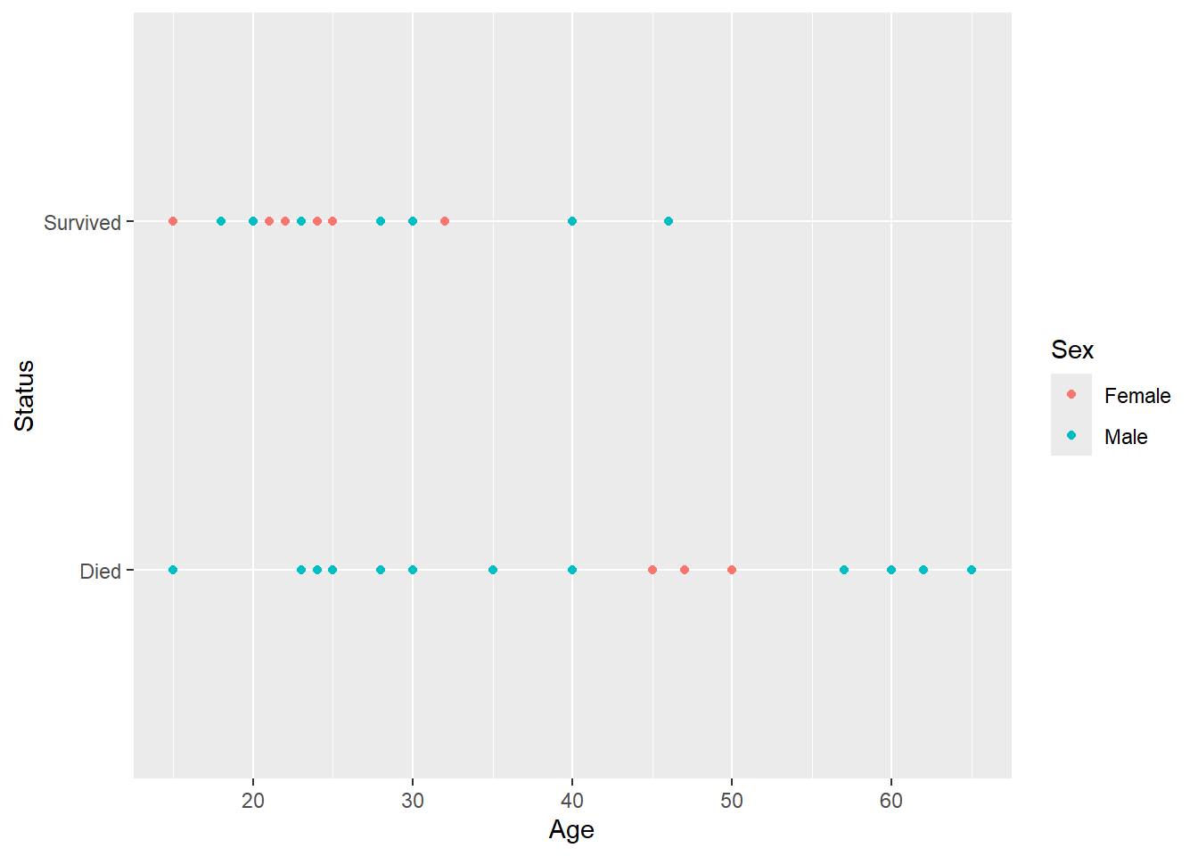
# Here's the code to fit a logistic regression model:

# Response ~ explanatory, data = data, family is new.
LRM = glm(Status~Age+Female,data=work,family=binomial(link="logit"))
summary(LRM)
Call:
glm(formula = Status ~ Age + Female, family = binomial(link = "logit"),
    data = work)

Coefficients:
            Estimate Std. Error z value Pr(>|z|)
(Intercept)  1.63312    1.11018   1.471   0.1413
Age         -0.07820    0.03728  -2.097   0.0359 *
Female       1.59729    0.75547   2.114   0.0345 *
---
Signif. codes:  0 '***' 0.001 '**' 0.01 '*' 0.05 '.' 0.1 ' ' 1

(Dispersion parameter for binomial family taken to be 1)

    Null deviance: 61.827  on 44  degrees of freedom
Residual deviance: 51.256  on 42  degrees of freedom
AIC: 57.256

Number of Fisher Scoring iterations: 4
# And approximate confidence intervals for the Beta's:
cis = confint.default(LRM)
cis 2.5 % 97.5 %
(Intercept) -0.5428002 3.809040837
Age -0.1512803 -0.005127799
Female 0.1166015 3.077985503exp(cis) 2.5 % 97.5 %
(Intercept) 0.5811187 45.1071530
Age 0.8596067 0.9948853
Female 1.1236716 21.7146143Drop in Deviance
The Drop in Deviance Test, analogous to extra sum of squares test in MLR. Drop in Deviance Using R
Use the drop in dev test to make inference about multiple regression coefficients.
This one includes a term for the interaction between Age and Female
Coefficients:
                Estimate    Std. Error    z value Pr(>|z|)
(Intercept)     0.31834     1.13103     0.281     0.7784
Age             -0.03248    0.03527     -0.921    0.3571
Female          6.92805     3.39887     2.038     0.0415
Age:Female      -0.16160    0.09426     -1.714    0.0865
The interaction term has no evidence, it’s different from zero. If we dropped age and interactions?
when you fit multiple linear regression models, you used the Extra sum of squares F test to compare models that differed by more than one explanatory variable. In logistic regression (and generalized linear modeling) we use the drop in deviance test
The drop in deviance test aka the likelihood ratio test:
Compare the max value of the likelihood fct in one model to another.
\(LRT = 2log(LMAX_{full} - 2log(LMAX_{reduced}))\)
When the reduced model is correct (i.e., under the null hypothesis), the LRT follows (approximately) a Chi-squared distribution with degrees of freedom equal to the difference in the number of parameters between the full and reduced models.
Most computer packages (including R) don’t report the
LMAX, but instead report a quantity called the deviance:
deviance = constant−2log(LMAX).
- Fortunately, the constant is the same for both the full and reduced models, so that:
\(LRT = deviance_{reduced} −deviance_{full}\)
Pass anove two models to do the test.
For the models:
- logit(pi) = β0 +β1Agei +β2Femalei +β3Agei : Femalei
- logit(pi) = β0 +β2Femalei
When using the anova function to compare models, the reduced (smaller) model goes first.
mod.full = glm(Status ~ Age*Female, data = work, family = binomial(link = "logit"))
mod.red = glm(Status ~ Female, data = work, family = binomial(link = "logit"))

anova(mod.red,mod.full)| Resid. Df | Resid. Dev | Df | Deviance | Pr(>Chi) |
|---|---|---|---|---|
| 43 | 57.28628 | NA | NA | NA |
| 41 | 47.34637 | 2 | 9.939909 | 0.0069435 |
Compare that drop in deviance statistic to a Chi-squrare distribution with 2 degrees of freedom
1-pchisq(9.93399,2)[1] 0.006964044p-value = 0.006964044, suggests there’s evidence to reject the reduced model in favor of the full model in this case.
Comparing this output to:
Coefficients:
                Estimate    Std. Error    z value Pr(>|z|)
(Intercept)     0.31834     1.13103     0.281     0.7784
Age             -0.03248    0.03527     -0.921    0.3571
Female          6.92805     3.39887     2.038     0.0415
Age:Female      -0.16160    0.09426     -1.714    0.0865
Shows that the interaction and age terms
Looking at the p-value for the int term, there isn’t evidence it’s different from zero, but the anova let’s us see that it is important.
Quizzes
R
All questions rely on the data in case1902 in the Sleuth3 library—you saw these data in Lab 1. The dataset contains sentencing outcomes (Death/NoDeath) from 362 murder trials in Georgia, as well as the race (Black/White) of the victim and aggravation level of the crime (1,2,…,6; where 6 is the most egregious). Use gather() or pivot_longer() and then expand.dft() to get the case1902 data into tidy (case) format. Feel free to refer to Lab 1
library(Sleuth3)
library(vcdExtra)
Loading required package: vcdLoading required package: gridLoading required package: gnm
Attaching package: 'vcdExtra'The following object is masked from 'package:dplyr':
summarisedata(case1902)df <- case1902
df <- df |> pivot_longer(cols = c(Death, NoDeath), names_to = "sent", values_to = "Freq")
df <- expand.dft(df)
df <- df |> mutate(
sent = ifelse(sent == "Death", 1, 0)
)
df| Aggravation | Victim | sent |
|---|---|---|
| 1 | White | 1 |
| 1 | White | 1 |
| 1 | White | 0 |
| 1 | White | 0 |
| 1 | White | 0 |
| 1 | White | 0 |
| 1 | White | 0 |
| 1 | White | 0 |
| 1 | White | 0 |
| 1 | White | 0 |
| 1 | White | 0 |
| 1 | White | 0 |
| 1 | White | 0 |
| 1 | White | 0 |
| 1 | White | 0 |
| 1 | White | 0 |
| 1 | White | 0 |
| 1 | White | 0 |
| 1 | White | 0 |
| 1 | White | 0 |
| 1 | White | 0 |
| 1 | White | 0 |
| 1 | White | 0 |
| 1 | White | 0 |
| 1 | White | 0 |
| 1 | White | 0 |
| 1 | White | 0 |
| 1 | White | 0 |
| 1 | White | 0 |
| 1 | White | 0 |
| 1 | White | 0 |
| 1 | White | 0 |
| 1 | White | 0 |
| 1 | White | 0 |
| 1 | White | 0 |
| 1 | White | 0 |
| 1 | White | 0 |
| 1 | White | 0 |
| 1 | White | 0 |
| 1 | White | 0 |
| 1 | White | 0 |
| 1 | White | 0 |
| 1 | White | 0 |
| 1 | White | 0 |
| 1 | White | 0 |
| 1 | White | 0 |
| 1 | White | 0 |
| 1 | White | 0 |
| 1 | White | 0 |
| 1 | White | 0 |
| 1 | White | 0 |
| 1 | White | 0 |
| 1 | White | 0 |
| 1 | White | 0 |
| 1 | White | 0 |
| 1 | White | 0 |
| 1 | White | 0 |
| 1 | White | 0 |
| 1 | White | 0 |
| 1 | White | 0 |
| 1 | White | 0 |
| 1 | White | 0 |
| 1 | Black | 1 |
| 1 | Black | 0 |
| 1 | Black | 0 |
| 1 | Black | 0 |
| 1 | Black | 0 |
| 1 | Black | 0 |
| 1 | Black | 0 |
| 1 | Black | 0 |
| 1 | Black | 0 |
| 1 | Black | 0 |
| 1 | Black | 0 |
| 1 | Black | 0 |
| 1 | Black | 0 |
| 1 | Black | 0 |
| 1 | Black | 0 |
| 1 | Black | 0 |
| 1 | Black | 0 |
| 1 | Black | 0 |
| 1 | Black | 0 |
| 1 | Black | 0 |
| 1 | Black | 0 |
| 1 | Black | 0 |
| 1 | Black | 0 |
| 1 | Black | 0 |
| 1 | Black | 0 |
| 1 | Black | 0 |
| 1 | Black | 0 |
| 1 | Black | 0 |
| 1 | Black | 0 |
| 1 | Black | 0 |
| 1 | Black | 0 |
| 1 | Black | 0 |
| 1 | Black | 0 |
| 1 | Black | 0 |
| 1 | Black | 0 |
| 1 | Black | 0 |
| 1 | Black | 0 |
| 1 | Black | 0 |
| 1 | Black | 0 |
| 1 | Black | 0 |
| 1 | Black | 0 |
| 1 | Black | 0 |
| 1 | Black | 0 |
| 1 | Black | 0 |
| 1 | Black | 0 |
| 1 | Black | 0 |
| 1 | Black | 0 |
| 1 | Black | 0 |
| 1 | Black | 0 |
| 1 | Black | 0 |
| 1 | Black | 0 |
| 1 | Black | 0 |
| 1 | Black | 0 |
| 1 | Black | 0 |
| 1 | Black | 0 |
| 1 | Black | 0 |
| 1 | Black | 0 |
| 1 | Black | 0 |
| 1 | Black | 0 |
| 1 | Black | 0 |
| 1 | Black | 0 |
| 1 | Black | 0 |
| 1 | Black | 0 |
| 1 | Black | 0 |
| 1 | Black | 0 |
| 1 | Black | 0 |
| 1 | Black | 0 |
| 1 | Black | 0 |
| 1 | Black | 0 |
| 1 | Black | 0 |
| 1 | Black | 0 |
| 1 | Black | 0 |
| 1 | Black | 0 |
| 1 | Black | 0 |
| 1 | Black | 0 |
| 1 | Black | 0 |
| 1 | Black | 0 |
| 1 | Black | 0 |
| 1 | Black | 0 |
| 1 | Black | 0 |
| 1 | Black | 0 |
| 1 | Black | 0 |
| 1 | Black | 0 |
| 1 | Black | 0 |
| 1 | Black | 0 |
| 1 | Black | 0 |
| 1 | Black | 0 |
| 1 | Black | 0 |
| 1 | Black | 0 |
| 1 | Black | 0 |
| 1 | Black | 0 |
| 1 | Black | 0 |
| 1 | Black | 0 |
| 1 | Black | 0 |
| 1 | Black | 0 |
| 1 | Black | 0 |
| 1 | Black | 0 |
| 1 | Black | 0 |
| 1 | Black | 0 |
| 1 | Black | 0 |
| 1 | Black | 0 |
| 1 | Black | 0 |
| 1 | Black | 0 |
| 1 | Black | 0 |
| 1 | Black | 0 |
| 1 | Black | 0 |
| 1 | Black | 0 |
| 1 | Black | 0 |
| 1 | Black | 0 |
| 1 | Black | 0 |
| 1 | Black | 0 |
| 1 | Black | 0 |
| 1 | Black | 0 |
| 1 | Black | 0 |
| 1 | Black | 0 |
| 1 | Black | 0 |
| 1 | Black | 0 |
| 1 | Black | 0 |
| 1 | Black | 0 |
| 1 | Black | 0 |
| 1 | Black | 0 |
| 1 | Black | 0 |
| 1 | Black | 0 |
| 1 | Black | 0 |
| 1 | Black | 0 |
| 1 | Black | 0 |
| 1 | Black | 0 |
| 1 | Black | 0 |
| 1 | Black | 0 |
| 1 | Black | 0 |
| 1 | Black | 0 |
| 1 | Black | 0 |
| 1 | Black | 0 |
| 1 | Black | 0 |
| 1 | Black | 0 |
| 1 | Black | 0 |
| 1 | Black | 0 |
| 1 | Black | 0 |
| 1 | Black | 0 |
| 1 | Black | 0 |
| 1 | Black | 0 |
| 1 | Black | 0 |
| 1 | Black | 0 |
| 1 | Black | 0 |
| 1 | Black | 0 |
| 1 | Black | 0 |
| 1 | Black | 0 |
| 1 | Black | 0 |
| 1 | Black | 0 |
| 1 | Black | 0 |
| 1 | Black | 0 |
| 1 | Black | 0 |
| 1 | Black | 0 |
| 1 | Black | 0 |
| 1 | Black | 0 |
| 1 | Black | 0 |
| 1 | Black | 0 |
| 1 | Black | 0 |
| 1 | Black | 0 |
| 1 | Black | 0 |
| 1 | Black | 0 |
| 1 | Black | 0 |
| 1 | Black | 0 |
| 1 | Black | 0 |
| 1 | Black | 0 |
| 1 | Black | 0 |
| 1 | Black | 0 |
| 1 | Black | 0 |
| 1 | Black | 0 |
| 1 | Black | 0 |
| 1 | Black | 0 |
| 1 | Black | 0 |
| 1 | Black | 0 |
| 1 | Black | 0 |
| 1 | Black | 0 |
| 1 | Black | 0 |
| 1 | Black | 0 |
| 1 | Black | 0 |
| 1 | Black | 0 |
| 1 | Black | 0 |
| 1 | Black | 0 |
| 1 | Black | 0 |
| 2 | White | 1 |
| 2 | White | 1 |
| 2 | White | 0 |
| 2 | White | 0 |
| 2 | White | 0 |
| 2 | White | 0 |
| 2 | White | 0 |
| 2 | White | 0 |
| 2 | White | 0 |
| 2 | White | 0 |
| 2 | White | 0 |
| 2 | White | 0 |
| 2 | White | 0 |
| 2 | White | 0 |
| 2 | White | 0 |
| 2 | White | 0 |
| 2 | White | 0 |
| 2 | Black | 1 |
| 2 | Black | 0 |
| 2 | Black | 0 |
| 2 | Black | 0 |
| 2 | Black | 0 |
| 2 | Black | 0 |
| 2 | Black | 0 |
| 2 | Black | 0 |
| 2 | Black | 0 |
| 2 | Black | 0 |
| 2 | Black | 0 |
| 2 | Black | 0 |
| 2 | Black | 0 |
| 2 | Black | 0 |
| 2 | Black | 0 |
| 2 | Black | 0 |
| 2 | Black | 0 |
| 2 | Black | 0 |
| 2 | Black | 0 |
| 2 | Black | 0 |
| 2 | Black | 0 |
| 2 | Black | 0 |
| 3 | White | 1 |
| 3 | White | 1 |
| 3 | White | 1 |
| 3 | White | 1 |
| 3 | White | 1 |
| 3 | White | 1 |
| 3 | White | 0 |
| 3 | White | 0 |
| 3 | White | 0 |
| 3 | White | 0 |
| 3 | White | 0 |
| 3 | White | 0 |
| 3 | White | 0 |
| 3 | Black | 1 |
| 3 | Black | 1 |
| 3 | Black | 0 |
| 3 | Black | 0 |
| 3 | Black | 0 |
| 3 | Black | 0 |
| 3 | Black | 0 |
| 3 | Black | 0 |
| 3 | Black | 0 |
| 3 | Black | 0 |
| 3 | Black | 0 |
| 4 | White | 1 |
| 4 | White | 1 |
| 4 | White | 1 |
| 4 | White | 1 |
| 4 | White | 1 |
| 4 | White | 1 |
| 4 | White | 1 |
| 4 | White | 1 |
| 4 | White | 1 |
| 4 | White | 0 |
| 4 | White | 0 |
| 4 | White | 0 |
| 4 | Black | 1 |
| 4 | Black | 1 |
| 4 | Black | 0 |
| 4 | Black | 0 |
| 4 | Black | 0 |
| 4 | Black | 0 |
| 5 | White | 1 |
| 5 | White | 1 |
| 5 | White | 1 |
| 5 | White | 1 |
| 5 | White | 1 |
| 5 | White | 1 |
| 5 | White | 1 |
| 5 | White | 1 |
| 5 | White | 1 |
| 5 | Black | 1 |
| 5 | Black | 1 |
| 5 | Black | 1 |
| 5 | Black | 1 |
| 5 | Black | 0 |
| 5 | Black | 0 |
| 5 | Black | 0 |
| 6 | White | 1 |
| 6 | White | 1 |
| 6 | White | 1 |
| 6 | White | 1 |
| 6 | White | 1 |
| 6 | White | 1 |
| 6 | White | 1 |
| 6 | White | 1 |
| 6 | White | 1 |
| 6 | White | 1 |
| 6 | White | 1 |
| 6 | White | 1 |
| 6 | White | 1 |
| 6 | White | 1 |
| 6 | White | 1 |
| 6 | White | 1 |
| 6 | White | 1 |
| 6 | Black | 1 |
| 6 | Black | 1 |
| 6 | Black | 1 |
| 6 | Black | 1 |
Use the glm() function to fit a logistic regression model that includes additive terms for Aggravation and Victim (e.g., Sentence ~ Aggravation + Victim ). What is the p-value corresponding to the coefficient on Victim?
0.000732
glm(sent ~ Aggravation + Victim,
    data = df,
    family = binomial(link = "logit")) |> summary()
Call:
glm(formula = sent ~ Aggravation + Victim, family = binomial(link = "logit"),
    data = df)

Coefficients:
            Estimate Std. Error z value Pr(>|z|)
(Intercept)  -6.6760     0.7574  -8.814  < 2e-16 ***
Aggravation   1.5397     0.1867   8.246  < 2e-16 ***
VictimWhite   1.8106     0.5361   3.377 0.000732 ***
---
Signif. codes:  0 '***' 0.001 '**' 0.01 '*' 0.05 '.' 0.1 ' ' 1

(Dispersion parameter for binomial family taken to be 1)

    Null deviance: 321.88  on 361  degrees of freedom
Residual deviance: 113.48  on 359  degrees of freedom
AIC: 119.48

Number of Fisher Scoring iterations: 7
Did the numeric algorithm used to obtain the maximum likelihood estimates of the logistic regression coefficients converge, and if so what evidence do you have for that.
It converged, the number of Fisher Scoring iterations is 7.
Which of the following statements best describes the odds of a Death sentence when the Victim was white relative to when the victim was black, for two murders at the same aggravation level?
Agg <- 0
White <- 1

# log(odds) = -6.6760 + 1.5397*Agg + 1.8106*White
odds1 = exp(-6.6760) + exp(1.8106*White)
odds1
[1] 6.115376White <- 0
odds2 = exp(-6.6760) + exp(1.8106*White)
odds2[1] 1.001261odds1/odds2[1] 6.107675The odds of a death sentence when the victim was white are estimated to be 6.11 times of the odds of a death sentence when the victim was black.
If you first make sure that the response variable, Sentence, is coded as 0 or 1, and then you use the glm() function on the death penalty data, but neglect to pass in the argument, “family=binomial” what happens?
df| Aggravation | Victim | sent |
|---|---|---|
| 1 | White | 1 |
| 1 | White | 1 |
| 1 | White | 0 |
| 1 | White | 0 |
| 1 | White | 0 |
| 1 | White | 0 |
| 1 | White | 0 |
| 1 | White | 0 |
| 1 | White | 0 |
| 1 | White | 0 |
| 1 | White | 0 |
| 1 | White | 0 |
| 1 | White | 0 |
| 1 | White | 0 |
| 1 | White | 0 |
| 1 | White | 0 |
| 1 | White | 0 |
| 1 | White | 0 |
| 1 | White | 0 |
| 1 | White | 0 |
| 1 | White | 0 |
| 1 | White | 0 |
| 1 | White | 0 |
| 1 | White | 0 |
| 1 | White | 0 |
| 1 | White | 0 |
| 1 | White | 0 |
| 1 | White | 0 |
| 1 | White | 0 |
| 1 | White | 0 |
| 1 | White | 0 |
| 1 | White | 0 |
| 1 | White | 0 |
| 1 | White | 0 |
| 1 | White | 0 |
| 1 | White | 0 |
| 1 | White | 0 |
| 1 | White | 0 |
| 1 | White | 0 |
| 1 | White | 0 |
| 1 | White | 0 |
| 1 | White | 0 |
| 1 | White | 0 |
| 1 | White | 0 |
| 1 | White | 0 |
| 1 | White | 0 |
| 1 | White | 0 |
| 1 | White | 0 |
| 1 | White | 0 |
| 1 | White | 0 |
| 1 | White | 0 |
| 1 | White | 0 |
| 1 | White | 0 |
| 1 | White | 0 |
| 1 | White | 0 |
| 1 | White | 0 |
| 1 | White | 0 |
| 1 | White | 0 |
| 1 | White | 0 |
| 1 | White | 0 |
| 1 | White | 0 |
| 1 | White | 0 |
| 1 | Black | 1 |
| 1 | Black | 0 |
| 1 | Black | 0 |
| 1 | Black | 0 |
| 1 | Black | 0 |
| 1 | Black | 0 |
| 1 | Black | 0 |
| 1 | Black | 0 |
| 1 | Black | 0 |
| 1 | Black | 0 |
| 1 | Black | 0 |
| 1 | Black | 0 |
| 1 | Black | 0 |
| 1 | Black | 0 |
| 1 | Black | 0 |
| 1 | Black | 0 |
| 1 | Black | 0 |
| 1 | Black | 0 |
| 1 | Black | 0 |
| 1 | Black | 0 |
| 1 | Black | 0 |
| 1 | Black | 0 |
| 1 | Black | 0 |
| 1 | Black | 0 |
| 1 | Black | 0 |
| 1 | Black | 0 |
| 1 | Black | 0 |
| 1 | Black | 0 |
| 1 | Black | 0 |
| 1 | Black | 0 |
| 1 | Black | 0 |
| 1 | Black | 0 |
| 1 | Black | 0 |
| 1 | Black | 0 |
| 1 | Black | 0 |
| 1 | Black | 0 |
| 1 | Black | 0 |
| 1 | Black | 0 |
| 1 | Black | 0 |
| 1 | Black | 0 |
| 1 | Black | 0 |
| 1 | Black | 0 |
| 1 | Black | 0 |
| 1 | Black | 0 |
| 1 | Black | 0 |
| 1 | Black | 0 |
| 1 | Black | 0 |
| 1 | Black | 0 |
| 1 | Black | 0 |
| 1 | Black | 0 |
| 1 | Black | 0 |
| 1 | Black | 0 |
| 1 | Black | 0 |
| 1 | Black | 0 |
| 1 | Black | 0 |
| 1 | Black | 0 |
| 1 | Black | 0 |
| 1 | Black | 0 |
| 1 | Black | 0 |
| 1 | Black | 0 |
| 1 | Black | 0 |
| 1 | Black | 0 |
| 1 | Black | 0 |
| 1 | Black | 0 |
| 1 | Black | 0 |
| 1 | Black | 0 |
| 1 | Black | 0 |
| 1 | Black | 0 |
| 1 | Black | 0 |
| 1 | Black | 0 |
| 1 | Black | 0 |
| 1 | Black | 0 |
| 1 | Black | 0 |
| 1 | Black | 0 |
| 1 | Black | 0 |
| 1 | Black | 0 |
| 1 | Black | 0 |
| 1 | Black | 0 |
| 1 | Black | 0 |
| 1 | Black | 0 |
| 1 | Black | 0 |
| 1 | Black | 0 |
| 1 | Black | 0 |
| 1 | Black | 0 |
| 1 | Black | 0 |
| 1 | Black | 0 |
| 1 | Black | 0 |
| 1 | Black | 0 |
| 1 | Black | 0 |
| 1 | Black | 0 |
| 1 | Black | 0 |
| 1 | Black | 0 |
| 1 | Black | 0 |
| 1 | Black | 0 |
| 1 | Black | 0 |
| 1 | Black | 0 |
| 1 | Black | 0 |
| 1 | Black | 0 |
| 1 | Black | 0 |
| 1 | Black | 0 |
| 1 | Black | 0 |
| 1 | Black | 0 |
| 1 | Black | 0 |
| 1 | Black | 0 |
| 1 | Black | 0 |
| 1 | Black | 0 |
| 1 | Black | 0 |
| 1 | Black | 0 |
| 1 | Black | 0 |
| 1 | Black | 0 |
| 1 | Black | 0 |
| 1 | Black | 0 |
| 1 | Black | 0 |
| 1 | Black | 0 |
| 1 | Black | 0 |
| 1 | Black | 0 |
| 1 | Black | 0 |
| 1 | Black | 0 |
| 1 | Black | 0 |
| 1 | Black | 0 |
| 1 | Black | 0 |
| 1 | Black | 0 |
| 1 | Black | 0 |
| 1 | Black | 0 |
| 1 | Black | 0 |
| 1 | Black | 0 |
| 1 | Black | 0 |
| 1 | Black | 0 |
| 1 | Black | 0 |
| 1 | Black | 0 |
| 1 | Black | 0 |
| 1 | Black | 0 |
| 1 | Black | 0 |
| 1 | Black | 0 |
| 1 | Black | 0 |
| 1 | Black | 0 |
| 1 | Black | 0 |
| 1 | Black | 0 |
| 1 | Black | 0 |
| 1 | Black | 0 |
| 1 | Black | 0 |
| 1 | Black | 0 |
| 1 | Black | 0 |
| 1 | Black | 0 |
| 1 | Black | 0 |
| 1 | Black | 0 |
| 1 | Black | 0 |
| 1 | Black | 0 |
| 1 | Black | 0 |
| 1 | Black | 0 |
| 1 | Black | 0 |
| 1 | Black | 0 |
| 1 | Black | 0 |
| 1 | Black | 0 |
| 1 | Black | 0 |
| 1 | Black | 0 |
| 1 | Black | 0 |
| 1 | Black | 0 |
| 1 | Black | 0 |
| 1 | Black | 0 |
| 1 | Black | 0 |
| 1 | Black | 0 |
| 1 | Black | 0 |
| 1 | Black | 0 |
| 1 | Black | 0 |
| 1 | Black | 0 |
| 1 | Black | 0 |
| 1 | Black | 0 |
| 1 | Black | 0 |
| 1 | Black | 0 |
| 1 | Black | 0 |
| 1 | Black | 0 |
| 1 | Black | 0 |
| 1 | Black | 0 |
| 1 | Black | 0 |
| 1 | Black | 0 |
| 1 | Black | 0 |
| 1 | Black | 0 |
| 1 | Black | 0 |
| 1 | Black | 0 |
| 1 | Black | 0 |
| 1 | Black | 0 |
| 2 | White | 1 |
| 2 | White | 1 |
| 2 | White | 0 |
| 2 | White | 0 |
| 2 | White | 0 |
| 2 | White | 0 |
| 2 | White | 0 |
| 2 | White | 0 |
| 2 | White | 0 |
| 2 | White | 0 |
| 2 | White | 0 |
| 2 | White | 0 |
| 2 | White | 0 |
| 2 | White | 0 |
| 2 | White | 0 |
| 2 | White | 0 |
| 2 | White | 0 |
| 2 | Black | 1 |
| 2 | Black | 0 |
| 2 | Black | 0 |
| 2 | Black | 0 |
| 2 | Black | 0 |
| 2 | Black | 0 |
| 2 | Black | 0 |
| 2 | Black | 0 |
| 2 | Black | 0 |
| 2 | Black | 0 |
| 2 | Black | 0 |
| 2 | Black | 0 |
| 2 | Black | 0 |
| 2 | Black | 0 |
| 2 | Black | 0 |
| 2 | Black | 0 |
| 2 | Black | 0 |
| 2 | Black | 0 |
| 2 | Black | 0 |
| 2 | Black | 0 |
| 2 | Black | 0 |
| 2 | Black | 0 |
| 3 | White | 1 |
| 3 | White | 1 |
| 3 | White | 1 |
| 3 | White | 1 |
| 3 | White | 1 |
| 3 | White | 1 |
| 3 | White | 0 |
| 3 | White | 0 |
| 3 | White | 0 |
| 3 | White | 0 |
| 3 | White | 0 |
| 3 | White | 0 |
| 3 | White | 0 |
| 3 | Black | 1 |
| 3 | Black | 1 |
| 3 | Black | 0 |
| 3 | Black | 0 |
| 3 | Black | 0 |
| 3 | Black | 0 |
| 3 | Black | 0 |
| 3 | Black | 0 |
| 3 | Black | 0 |
| 3 | Black | 0 |
| 3 | Black | 0 |
| 4 | White | 1 |
| 4 | White | 1 |
| 4 | White | 1 |
| 4 | White | 1 |
| 4 | White | 1 |
| 4 | White | 1 |
| 4 | White | 1 |
| 4 | White | 1 |
| 4 | White | 1 |
| 4 | White | 0 |
| 4 | White | 0 |
| 4 | White | 0 |
| 4 | Black | 1 |
| 4 | Black | 1 |
| 4 | Black | 0 |
| 4 | Black | 0 |
| 4 | Black | 0 |
| 4 | Black | 0 |
| 5 | White | 1 |
| 5 | White | 1 |
| 5 | White | 1 |
| 5 | White | 1 |
| 5 | White | 1 |
| 5 | White | 1 |
| 5 | White | 1 |
| 5 | White | 1 |
| 5 | White | 1 |
| 5 | Black | 1 |
| 5 | Black | 1 |
| 5 | Black | 1 |
| 5 | Black | 1 |
| 5 | Black | 0 |
| 5 | Black | 0 |
| 5 | Black | 0 |
| 6 | White | 1 |
| 6 | White | 1 |
| 6 | White | 1 |
| 6 | White | 1 |
| 6 | White | 1 |
| 6 | White | 1 |
| 6 | White | 1 |
| 6 | White | 1 |
| 6 | White | 1 |
| 6 | White | 1 |
| 6 | White | 1 |
| 6 | White | 1 |
| 6 | White | 1 |
| 6 | White | 1 |
| 6 | White | 1 |
| 6 | White | 1 |
| 6 | White | 1 |
| 6 | Black | 1 |
| 6 | Black | 1 |
| 6 | Black | 1 |
| 6 | Black | 1 |
glm(sent ~ Aggravation + Victim,
    data = df) |> summary()
Call:
glm(formula = sent ~ Aggravation + Victim, data = df)

Coefficients:
             Estimate Std. Error t value Pr(>|t|)
(Intercept) -0.212931   0.019125 -11.134  < 2e-16 ***
Aggravation  0.185380   0.008332  22.249  < 2e-16 ***
VictimWhite  0.088504   0.026020   3.401 0.000746 ***
---
Signif. codes:  0 '***' 0.001 '**' 0.01 '*' 0.05 '.' 0.1 ' ' 1

(Dispersion parameter for gaussian family taken to be 0.04985609)

    Null deviance: 49.384  on 361  degrees of freedom
Residual deviance: 17.898  on 359  degrees of freedom
AIC: -53.2

Number of Fisher Scoring iterations: 2
A logistic regression model is fit, but it uses Normal (Gaussian) errors.
- A multiple linear regression model is fit by default.
C
All four questions on this quiz are related to the situation and output provided here:
On January 28, 1986, a routine launch was anticipated for the Challenger space shuttle. Seventy-three seconds into the flight, disaster happened: the shuttle broke apart, killing all seven crew members on board. An investigation into the cause of the disaster focused on a critical seal called an O-ring, and it is believed that damage to O-rings during shuttle launches may have been related to the ambient temperature at the time of the launch. Using data from 24 shuttle missions, we fit a simple logistic regression model. Here, Temperature is the temperature in Fahrenheit at launch time and the response variable, Failure, is an indicator of O-rings failures (Failure = 1 if there was at least O-ring that failed.)
Here is a summary of the logistic regression model t to these data:
Estimate    Std. Error  z value Pr(>|z|
(Intercept) 10.88   5.70    1.91    0.06
Temperature -0.17   0.08    -2.05   0.04
1.
Give a 95% confidence interval for the coefficient on Temperature.
Ans c(-17 - 1.96(.08), -17 + 1.96(.08))
c((-.17 - 1.96*(.08)), (-.17 + 1.96*(.08)))[1] -0.3268 -0.0132t <- -.17
se <- .08
z <- 2.05
c(t - se*z, t+se*z)[1] -0.334 -0.006(-0.33, -0.01)
2.
In the context of the problem, is this the correct interpretation of the confidence interval you found in question 1, on the log-odds scale. (True or False)
A one degree increase in temperature is associated with an estimated decrease in the log odds of O-ring failure between 0.0132 and 0.3268 (95% confidence interval for the log-odds of failure).
ANS, TRUE
0.0132 - 0.3268[1] -0.31363.
Give a 95% confidence interval for the effect of a one-degree increase in temperature on the odds of O-ring failure.
ANS c(exp(-17 - 1.96(.08)), exp(-17 + 1.96(.08))
c((exp(-.17 - 1.96*(.08))), exp(-.17 + 1.96*(.08)))[1] 0.7212280 0.9868867(10.88 + (5.7*1.91))[1] 21.767(10.88 -.17 + (5.7*1.91) + (.08 * -2.05))[1] 21.433(10.88 + (5.7*1.91))- (10.88 -.17 + (5.7*1.91) + (.08 * -2.05))[1] 0.334(10.88)[1] 10.88(10.88 - .17)[1] 10.71(10.88) - (10.88 - .17)[1] 0.17exp(0.0132) [1] 1.013288exp(0.3268)[1] 1.3865244.
In the context of the problem, is this the correct interpretation of the confidence interval you found in question 3. (True or False)
We estimate that the odds of O-ring failure decrease between roughly 72% and 99% for each one degree increase in temperature (95% confidence interval for the odds of O-ring failure).
TRUE
We estimate that the odds of O-ring failure decrease between roughly 72% and 99% for each one degree increase in temperature (95% confidence interval for the odds of O-ring failure).
Discussion
Maximum Likelihood.
Logistic function from zero to one shows probability between zero and one.
We can only test to see if a variables effect is different from zero with walds test.
In linear regression we fit a line with least squares.
Here we use maximum likelihood. Pick a probability curve scaled by x of observing a 1. Use that to calculate a likelihood of observing a zero at x, and do that for every x,y combo, then multiply all likelihoods together. That is the likelihood of the data, given the line. Shift the line and repeat iteratively. The curve with the maximum likelihood wins.
Log reg can be used to classify samples. It can use different types of data, and can assess what variables were useful to classify the sample.
Maximum Likelihood.
The goal is to find the optimal way to fit a distribution to the data. To do this, try fitting a distribution to the data. Measure the probability/likelihood of observing the data with the distribution at that point, then move the distribution and try again. Pick the point in the set maximizes the probability/likelihood of observing the values.
library(tidyverse)
p <- .8
X <- 0:99
x1 <- 19
x2 <- 20
successes <- rep(1,p*length(X))
failures <- rep(0,((1 - p)*(length(X)) + 1))
y1 <- 0
y2 <- 1
m <- ((y2 - y1)/(x2 - x1))
b <- y1 - m*x1
y = m*(X - x1) + y1
logodds <- y
prob <- exp(logodds)/(1 + exp(logodds))
data <- c(failures, successes)
ggplot() +
aes(x = X, y = data) +
geom_point() +
geom_abline(intercept = b, slope = m, color = "blue") +
# geom_point(aes(x = x, y = logodds), color = "blue") +
labs(title = "Log odds is y of blue dots") +
geom_point(aes(x = X, y = prob), color = "red") +
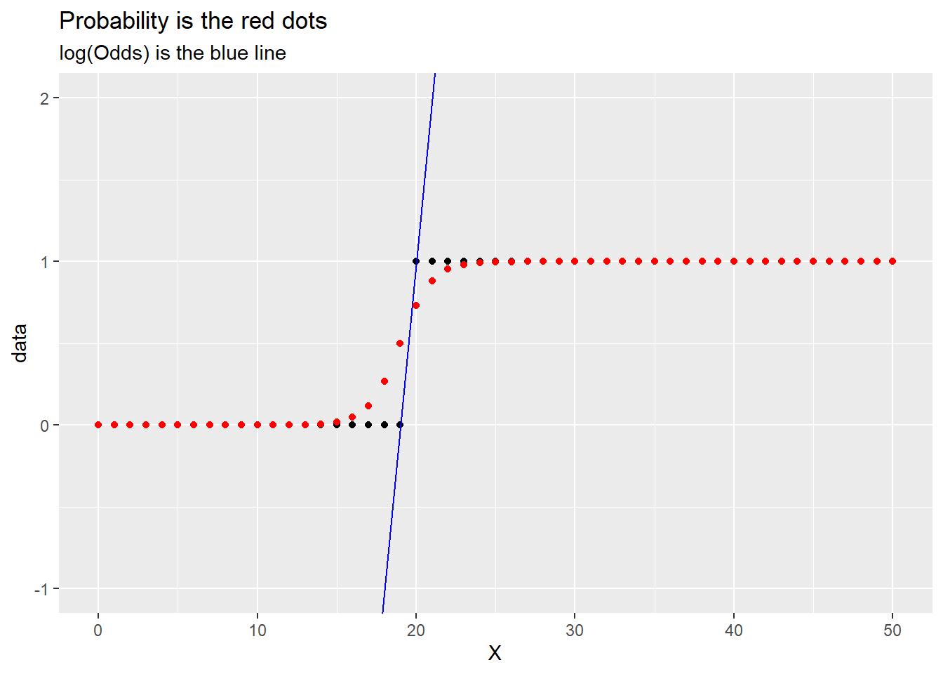
labs(title = "Probability is the red dots",
subtitle = "log(Odds) is the blue line") +
ylim(c(-1,2)) +
xlim(c(0, 50))Warning: Removed 49 rows containing missing values or values outside the scale range
(`geom_point()`).
Removed 49 rows containing missing values or values outside the scale range
(`geom_point()`).