ST-518 HW 4

Author

Chris Eckerson

Published

May 17, 2024

R Question

1. Spock trial

(5 points) In 1968, Dr. Benjamin Spock was tried in Boston on charges of conspiring to violate the Selective Service Act by encouraging young men to resist the draft for military service in Vietnam. The defense in the case challenged the method of jury selection claiming that women were underrepresented on jury panels by the process. The defense argued specifically that the judge in the Spock trial had a history of venires (panels of potential jurors) in which women were systematically underrepresented compared to the venires of six other Boston area district judges. These data can be found in case0502 in the Sleuth3 package.

Analyze the data by treating the number of women out of 30 people on a venire as a binomial response (that is, you’ll change the percent women in the datasheet to a count by multiplying by 30 and rounding) and judge as an explanatory variable.

Re-write- Defense claims women are underrepresented on jury. case0502

a. Over dispersion

  1. Is there evidence of over dispersion in these data? Please explain (i.e., don’t just answer “yes” or “no”).
rm(list = ls())

logistic <- function(x) {(exp(x))/(1 + exp(x))}
data("case0502")
df <- case0502

df <- df |> group_by(Judge) |> mutate(
    venire_id = row_number(),
    prop = Percent/100, 
    n = 30, 
    female = round(prop*n),
    male = n - female) |> ungroup()

df1 <- df |> dplyr::select(Judge, female, n)

df |> head(n = 10)
Percent Judge venire_id prop n female male
6.4 Spock’s 1 0.064 30 2 28
8.7 Spock’s 2 0.087 30 3 27
13.3 Spock’s 3 0.133 30 4 26
13.6 Spock’s 4 0.136 30 4 26
15.0 Spock’s 5 0.150 30 4 26
15.2 Spock’s 6 0.152 30 5 25
17.7 Spock’s 7 0.177 30 5 25
18.6 Spock’s 8 0.186 30 6 24
23.1 Spock’s 9 0.231 30 7 23
16.8 A 1 0.168 30 5 25
emplog <- with(df, qlogis((female/n)))
m1 <- glm((female/n)~Judge, 
          weights = n,
    data = df1, 
    family = "binomial") 

m1 |> summary()

Call:
glm(formula = (female/n) ~ Judge, family = "binomial", data = df1, 
    weights = n)

Coefficients:
             Estimate Std. Error z value Pr(>|z|)    
(Intercept)  -0.66329    0.17236  -3.848 0.000119 ***
JudgeB        0.01974    0.23305   0.085 0.932484    
JudgeC       -0.23749    0.21849  -1.087 0.277049    
JudgeD       -0.34831    0.33902  -1.027 0.304239    
JudgeE       -0.37691    0.24188  -1.558 0.119171    
JudgeF       -0.32945    0.22019  -1.496 0.134599    
JudgeSpock's -1.08591    0.24302  -4.468 7.88e-06 ***
---
Signif. codes:  0 '***' 0.001 '**' 0.01 '*' 0.05 '.' 0.1 ' ' 1

(Dispersion parameter for binomial family taken to be 1)

    Null deviance: 62.919  on 45  degrees of freedom
Residual deviance: 31.119  on 39  degrees of freedom
AIC: 208.53

Number of Fisher Scoring iterations: 4
31.119/39
[1] 0.7979231

Psi is estimated to be less than 1, therefore there is no evidence of over-dispersion.

I am confused on these models, the examples always have a continuous explanatory variables, but here we don’t

b. Odds of female by judge

Hint: In parts (b) through (d), think about what models you could compare using drop-in-deviance tests.

  1. Do the odds of a female on a venire differ for the different judges? Please explain.
m1 <- glm((female/n)~Judge, 
          weights = n,
          data = df1, 
          family = "binomial") 

s1 <- summary(m1)
s1$coefficients
                Estimate Std. Error    z value     Pr(>|z|)
(Intercept)  -0.66329422  0.1723626 -3.8482499 1.189647e-04
JudgeB        0.01974398  0.2330503  0.0847198 9.324842e-01
JudgeC       -0.23749233  0.2184896 -1.0869732 2.770486e-01
JudgeD       -0.34830669  0.3390223 -1.0273858 3.042389e-01
JudgeE       -0.37690731  0.2418765 -1.5582634 1.191708e-01
JudgeF       -0.32945007  0.2201900 -1.4962083 1.345994e-01
JudgeSpock's -1.08590564  0.2430158 -4.4684570 7.878583e-06

\[ log(odds) = -0.66329422A + 0.01974398B -0.23749233C -0.34830669D -0.37690731E -0.32945007F -1.08590564S \] All the variables are dummy variables. Meaning each coefficient is also the log odds for that judge.

log_odds <- function(A,B,C,D,E,f,S) {
   log_o = -0.66329422*A + 0.01974398*B -0.23749233*C -0.34830669*D -0.37690731*E -0.32945007*f -1.08590564*S
   odds = exp(log_o)
   odds
  }

odds_a <- log_odds(1,0,0,0,0,0,0)
odds_a^(-1)
[1] 1.941176
odds_a <- log_odds(1,1,0,0,0,0,0)
odds_a^(-1)
[1] 1.903226
odds_a <- log_odds(1,0,1,0,0,0,0)
odds_a^(-1)
[1] 2.461538
odds_a <- log_odds(1,0,0,1,0,0,0)
odds_a^(-1)
[1] 2.75
odds_a <- log_odds(1,0,0,0,1,0,0)
odds_a^(-1)
[1] 2.829787
odds_a <- log_odds(1,0,0,0,0,1,0)
odds_a^(-1)
[1] 2.69863
odds_s <- log_odds(1,0,0,0,0,0,1)
odds_s^(-1)
[1] 5.75

The odds of being on each judges venire are : All in favor of choosing a male and against 1

  • A: 1.941176
  • B: 1.903226
  • C: 2.461538
  • D: 2.75
  • E: 2.829787
  • f: 2.69863
  • Spock: 5.75

Spock is estimated to be more likely to favor males.

ci1 <- confint.default(m1)
ci1 |> exp()
                 2.5 %    97.5 %
(Intercept)  0.3674681 0.7221880
JudgeB       0.6459544 1.6104510
JudgeC       0.5139013 1.2101440
JudgeD       0.3632085 1.3718563
JudgeE       0.4269977 1.1020388
JudgeF       0.4671922 1.1075101
JudgeSpock's 0.2096726 0.5435664

The multiplicative confidence intervals seem to tell the same story. Judges B through F potentially have the same odds of picking females as Judge A. However, Spock’s odds are between 21% and 54% the odds of A.
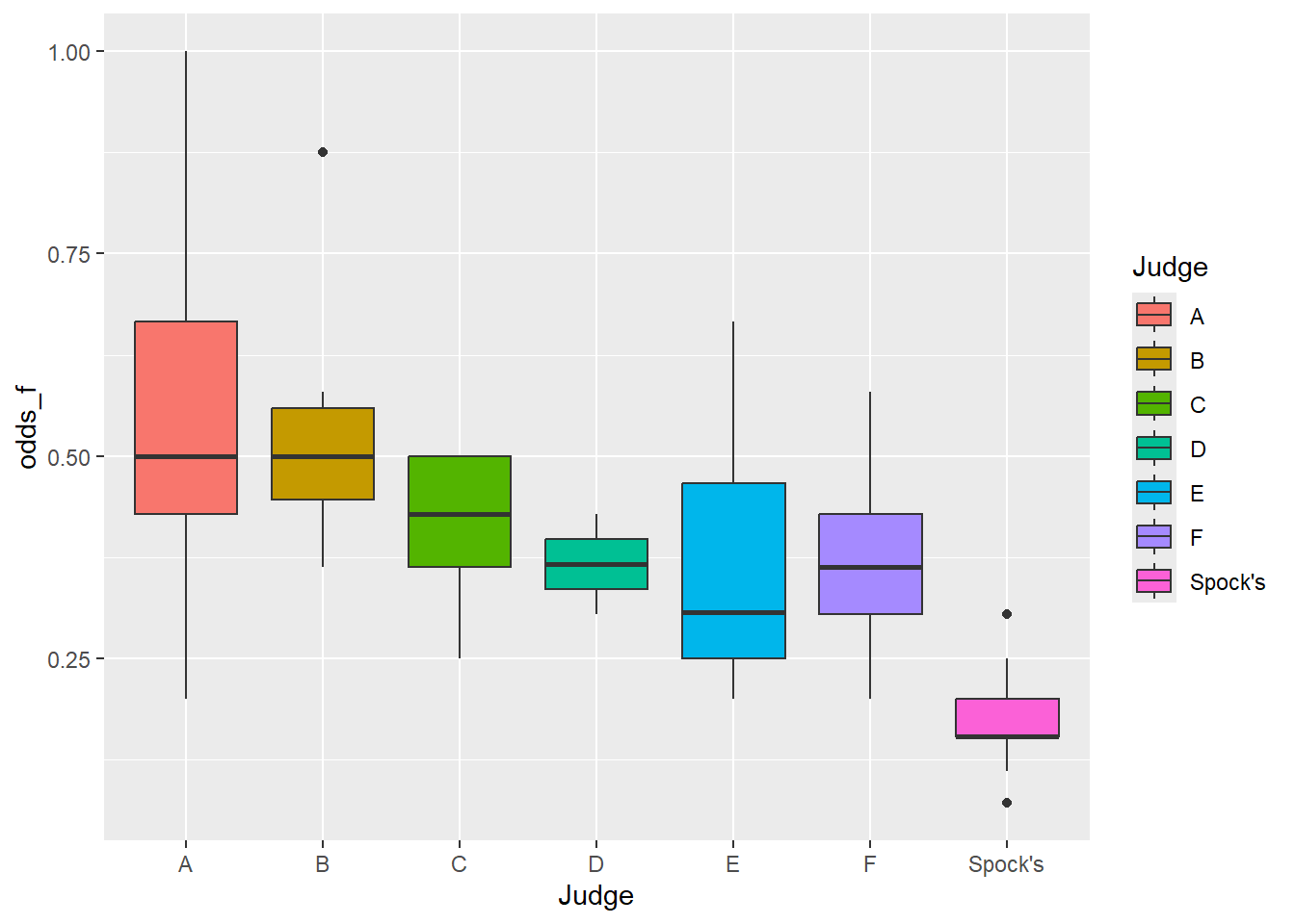
df4 <- df1 |> mutate(
  prop_f = female/n, 
  odds_f = ((prop_f)/(1 - prop_f)
))


ggplot(df4) +
  aes(x = Judge, y = odds_f, fill = Judge) +
  geom_boxplot()

Graphically, it is more obvious that there is a difference between the judges. Spock is the most obvious difference.

anova

dfanova <- df1 |> mutate(
  tot = n,
  male = tot - female,
  j = 1
) 


t <- dfanova |> 
  mutate(
    id = row_number()) |> 
  pivot_wider(names_from = Judge, 
                   values_from = j, 
                   id_cols = c(id, female, male, tot),
                   values_fill = 0) |> rename(S = `Spock's`, f = 'F') |> 
  relocate(S, .after = "f")

mf <- glm((female/tot)~B+C+D+E+f+S, 
          weights = tot,
    data = t, 
    family = "binomial") 


ms <-  glm((female/tot)~B+C+D+E+f, 
            weights = tot,
            data = t, 
            family = "binomial") 

mF <-  glm((female/tot)~B+C+D+E+S, 
            weights = tot,
            data = t, 
            family = "binomial") 


me <-  glm((female/tot)~B+C+D+f+S, 
            weights = tot,
            data = t, 
            family = "binomial") 

md <-  glm((female/tot)~B+C+E+f+S, 
            weights = tot,
            data = t, 
            family = "binomial") 


mc <-  glm((female/tot)~B+D+E+f+S, 
            weights = tot,
            data = t, 
            family = "binomial") 


mb <-  glm((female/tot)~C+D+E+f+S, 
            weights = tot,
            data = t, 
            family = "binomial") 

mods <- c('ms', 'mF', 'me', 'md', 'mc', 'mb')
for (i in 1:6) {
  print(mods[i])
  name <- get(mods[i])
  print(pchisq((anova(name, mf)$Deviance[2]), 1, lower.tail = F))
}
[1] "ms"
[1] 6.975788e-06
[1] "mF"
[1] 0.136041
[1] "me"
[1] 0.1188039
[1] "md"
[1] 0.2981783
[1] "mc"
[1] 0.2784756
[1] "mb"
[1] 0.9324773

The model without Spock is the only one that rejects the null hypothesis that the coefficients are equal. The full model, with Spock, is a better fit. The factor “Spock’s” is not equal to zero, Spock is different than the others.

c. Judges A-F

think about what models you could compare using drop-in-deviance tests.

  1. Do judges A-F differ in their probabilities of selecting females to the venire? Please explain.
dfc <- df |> filter(Judge != "Spock's")
m2 <- glm((female/n)~Judge, 
          weights = n,
    data = dfc, 
    family = "binomial") 

s2 <- summary(m2)
s2

Call:
glm(formula = (female/n) ~ Judge, family = "binomial", data = dfc, 
    weights = n)

Coefficients:
            Estimate Std. Error z value Pr(>|z|)    
(Intercept) -0.66329    0.17236  -3.848 0.000119 ***
JudgeB       0.01974    0.23305   0.085 0.932484    
JudgeC      -0.23749    0.21849  -1.087 0.277049    
JudgeD      -0.34831    0.33902  -1.027 0.304239    
JudgeE      -0.37691    0.24188  -1.558 0.119171    
JudgeF      -0.32945    0.22019  -1.496 0.134599    
---
Signif. codes:  0 '***' 0.001 '**' 0.01 '*' 0.05 '.' 0.1 ' ' 1

(Dispersion parameter for binomial family taken to be 1)

    Null deviance: 31.747  on 36  degrees of freedom
Residual deviance: 26.168  on 31  degrees of freedom
AIC: 173.19

Number of Fisher Scoring iterations: 4
s2$coefficients |> exp()
             Estimate Std. Error    z value Pr(>|z|)
(Intercept) 0.5151515   1.188109 0.02131701 1.000119
JudgeB      1.0199402   1.262445 1.08841205 2.540813
JudgeC      0.7886029   1.244196 0.33723569 1.319231
JudgeD      0.7058824   1.403575 0.35794148 1.355593
JudgeE      0.6859797   1.273637 0.21050131 1.126562
JudgeF      0.7193192   1.246313 0.22397781 1.144078
c2 <- confint.default(m2) 
c2
                 2.5 %      97.5 %
(Intercept) -1.0011186 -0.32546980
JudgeB      -0.4370263  0.47651425
JudgeC      -0.6657240  0.19073939
JudgeD      -1.0127782  0.31616482
JudgeE      -0.8509766  0.09716194
JudgeF      -0.7610145  0.10211435
c2 |> exp()
                2.5 %   97.5 %
(Intercept) 0.3674681 0.722188
JudgeB      0.6459544 1.610451
JudgeC      0.5139013 1.210144
JudgeD      0.3632085 1.371856
JudgeE      0.4269977 1.102039
JudgeF      0.4671922 1.107510

There may be differences between judges A through F, but the 95% confidence intervals seem to indicate that it is plausible that these judges all have roughly to same odds of choosing females. The confidence intervals contain 1 and they are multiplicative off of A. Meaning judges B through F are all choosing at roughly the same rate.

# -0.66329422  0.01974398 -0.23749233 -0.34830669 -0.37690731 -0.32945007
log_odds <- function(A,B,C,D,E,f) {
   log_o = (-0.66329422*A) + (0.01974398*B) + (-0.23749233*C) + (-0.34830669*D) + (-0.37690731*E) + (-0.32945007*f)
   odds = exp(log_o)
   odds
  }

odds_a <- log_odds(1,0,0,0,0,0)
odds_a^(-1)
[1] 1.941176
odds_a <- log_odds(1,1,0,0,0,0)
odds_a^(-1)
[1] 1.903226
odds_a <- log_odds(1,0,1,0,0,0)
odds_a^(-1)
[1] 2.461538
odds_a <- log_odds(1,0,0,1,0,0)
odds_a^(-1)
[1] 2.75
odds_a <- log_odds(1,0,0,0,1,0)
odds_a^(-1)
[1] 2.829787
odds_a <- log_odds(1,0,0,0,0,1)
odds_a^(-1)
[1] 2.69863

The odds for these judges range from about 1.9 to 2.8 in favor of males.

anova

dfanova <- df1 |> mutate(
  tot = n,
  male = tot - female,
  j = 1
) |> filter(Judge != "Spock's")


t <- dfanova |> 
  mutate(
    id = row_number()) |> 
  pivot_wider(names_from = Judge, 
              values_from = j, 
              id_cols = c(id, female, male, tot),
              values_fill = 0) |> rename(f = 'F') 

mf <- glm((female/tot)~B+C+D+E+f, 
          weights = tot,
    data = t, 
    family = "binomial") 


# ms <-  glm((female/tot)~B+C+D+E+f, 
#             weights = tot,
#             data = t, 
#             family = "binomial") 

mF <-  glm((female/tot)~B+C+D+E, 
            weights = tot,
            data = t, 
            family = "binomial") 


me <-  glm((female/tot)~B+C+D+f, 
            weights = tot,
            data = t, 
            family = "binomial") 

md <-  glm((female/tot)~B+C+E+f, 
            weights = tot,
            data = t, 
            family = "binomial") 


mc <-  glm((female/tot)~B+D+E+f, 
            weights = tot,
            data = t, 
            family = "binomial") 


mb <-  glm((female/tot)~C+D+E+f, 
            weights = tot,
            data = t, 
            family = "binomial") 

mods <- c('mF', 'me', 'md', 'mc', 'mb')
for (i in 1:length(mods)) {
  print(mods[i])
  name <- get(mods[i])
  print(pchisq((anova(name, mf)$Deviance[2]), 1, lower.tail = F))
}
[1] "mF"
[1] 0.136041
[1] "me"
[1] 0.1188039
[1] "md"
[1] 0.2981783
[1] "mc"
[1] 0.2784756
[1] "mb"
[1] 0.9324773

Testing the remaining judges, the all fail to reject the null hypothesis. Judges A though F are equally likely to choose females.

d. Spock v everyone.

  1. How different are the odds of having a woman on the Spock judge’s venires from the odds of having a woman on the venires of other judges? Please explain.

think about what models you could compare using drop-in-deviance tests.

As stated in part B, the odds of being on each judges venire are : All in favor of choosing a male and against 1

  • A: 1.941176
  • B: 1.903226
  • C: 2.461538
  • D: 2.75
  • E: 2.829787
  • f: 2.69863
  • Spock: 5.75

Comparing the ratios of the odds of Spock choosing a female vs the other judges,

5.75/ 1.941176
[1] 2.962122
5.75/ 1.903226
[1] 3.021186
5.75/ 2.461538
[1] 2.335938
5.75/ 2.75
[1] 2.090909
5.75/ 2.829787
[1] 2.031955
5.75/ 2.69863
[1] 2.130711
5.75/ 5.75
[1] 1

Spock is about:

  • 3 times more likely to choose male than A,
  • 3 times more likely than B,
  • 2.33 times more likely than C,
  • 2.1 times more likely than D,
  • 2.0 times more likely than E, and
  • 2.1 times more likely than F.

The ANOVA in parts b and c showed that Spock is the only judge that is significantly different among this group. (Drop in Deviance test, P-value = 6.975788e-06 on 1 df).

Conceptual Questions

2. Extra-binomial variation

(2 points) Give three explanations for why you may see evidence of extra-binomial variation in a logistic regression.

Extra-binomial variation could come from variables not represented in the model, outliers, or lack of independence. Unrepresented variables add noise because we are not predicting for their effect. Outliers are noise and come from a variety of sources, sometimes they are just mistakes, but they could be natural. Lack of independence causes observations to be more alike, that makes variation estimates low.

3. Misleading results

(2 points) In lecture, we saw that when we fit a logistic model when extra binomial variation is present, we get standard errors that are ’too small’. Explain why this gives misleading results.

If the data have more variation than is estimated in the model, the standard errors will be too small and confidence intervals too narrow. Variation in a binomial is p(1-p). If the data are not truly from a binomial distribution and there is a larger spread, then that equation is wrong.

4. Distribution of insects surviving

(1 point) Consider an experiment that studies the number of insects that survive a certain dose of an insecticide, using several batches of insects of size n each. The insects may be sensitive to factors that vary among batches during the experiment but these factors (such as temperature) were unmeasured. Explain why the distribution of the number of insects per batch surviving the experiment might show over dispersion relative to a binomial(n, p) distribution.

The insects in each batch are not independent of one another, they live together. Furthermore, each batch of insects is subject to unmeasured variables that are not in the model.