8 Model Eval

Learning Objectives

At the end of this week you should be able to:

Discuss issues having to with making predictions of binary outcomes
Describe methods for prediction of categorical and count data
Describe the statistical concerns to be aware of in the big data setting

In R:

Make predictions from generalized linear models
Evaluate different models using cross validation methods
Prepare and submit an R markdown script.

Task list

In order to achieve these learning outcomes, please make sure to complete the following:

~~Module 8 Readings~~
~~Lectures~~
~~Module 8 Lab~~
Module 8 Homework
~~R Quiz~~
~~Content Quiz~~
~~Discussion Wed~~
~~Disc Sunday~~

library(tidyverse)
# Classifier example libs. 
library(openintro)
library(vcdExtra)
library(ggplot2)
library(tidyverse)
library(magrittr)
library(boot)
library(pROC)

8 Model Eval Lectures

Binary Classification

Looking at the email dataset and the binary classification problem.

email dataset from openintro stats in mod 3
3921 emails in one account
21 variables for each email.
spam or not prediction.

Simple start

74% training set.
fit log reg using spam as response
to_multiple as exp
model is logit(p) = -2.1 -2.11 x multiple
Back transforms the equation to find p of spam or not.

If an incoming email is addressed to multiple people, then the estimated probability that it’s spam is 0.015 and if it’s not addressed to multiple people, then the estimated probability that it’s spam is 0.109.

We don’t just want probs, we want to classify/predict.

for ex, if prob > .5 it’s spam, or .75, whatever
here the probs are low and those numbers won’t work.
we need a better prediction model and
we need to figure out a classification rule.

Comparing Predictions

Mean Squared Prediction Errors & Receiver Operating Characteristic Curves (ROC curves)

good means predictions are right
how good depends on situation. Health would need to be more strict than spam.
pred error is difference yhat and y
we held back 25% for that.
MSPE = Mean Squared Prediction Error

\(MSPE = 1/m \sum{(\hat{y_i} −y_i)^2}\)

m is the number of values in a validation dataset.
For binary outcomes MSPE is prop of incorrect predictions, bc each squared pred err is zero or one.
smaller error is a better model.
We want to pick the model/classification rule combination that minimizes MSPE

ROC curves.

ROC is a graphical tool to evaluate a pred model with different classification rules.
false positive rate fpr is prob of predicting 1 when zero
true pos rate tpr is prob of pred 1 when 1.
we want to minimize fpr and max tpr.
ROC is tpr ~ fpr
1 to 1 is even chance.
more above the 1:1 line is better.
the point furthest from the 1:1 line that maxes and mins the rates is the number above which we set the rule.

Specificity = 1 - fpr

sensitivity = tpr

Specificity or sensitivity could be on the ROC curve instead. i.e. R does that.

Classifier Example

# ?email
names(email)

 [1] "spam"         "to_multiple"  "from"         "cc"           "sent_email"  
 [6] "time"         "image"        "attach"       "dollar"       "winner"      
[11] "inherit"      "viagra"       "password"     "num_char"     "line_breaks" 
[16] "format"       "re_subj"      "exclaim_subj" "urgent_subj"  "exclaim_mess"
[21] "number"

Training & Test Sets

Sample 75% of the email dataset, perform a simple logistic regression.

# simple log reg
(n <- dim(email)[1]) # num of obs in dataset

[1] 3921

(r <- round(n*.75)) # .75 for training data

[1] 2941

idx <- 1:n # index of all rows from 1 to n
nidx <- sample(idx,r,replace=F) # sample from index of .75
email75 <- email[nidx,] # set training
email25 <- email[-nidx,] # set test set
# set simple glm
pmod1 <- glm(spam~to_multiple,data=email75,family=binomial)
summary(pmod1)


Call:
glm(formula = spam ~ to_multiple, family = binomial, data = email75)

Coefficients:
             Estimate Std. Error z value Pr(>|z|)    
(Intercept)  -2.12057    0.06501 -32.619  < 2e-16 ***
to_multiple1 -2.06475    0.38619  -5.346 8.97e-08 ***
---
Signif. codes:  0 '***' 0.001 '**' 0.01 '*' 0.05 '.' 0.1 ' ' 1

(Dispersion parameter for binomial family taken to be 1)

    Null deviance: 1813.1  on 2940  degrees of freedom
Residual deviance: 1757.2  on 2939  degrees of freedom
AIC: 1761.2

Number of Fisher Scoring iterations: 6

Predictions

Get predictions for the model;

pred <- predict.glm(pmod1,newdata = email25, type="link") # get predictions
phat <- plogis(pred) # get preds on probability scale.

Now, we need a classifier rule to take these probabilities and turn them into 0’s and 1’s. Let’s just use:

ytilde <- ifelse(phat >= 0.50,1,0) # setting naive classifier rule
# and then calculate MSPE:
(MSPE1 <- mean((ytilde-(as.integer(email25$spam)-1))^2))

[1] 0.09693878

That’s actually not a bad mis-classification rate, but the reason is really that there are not that many spam emails!

(mean(as.integer(email25$spam)-1))

[1] 0.09693878

This is exactly the same as the MSPE, because our classification rule classified everything in email25 as non-spam! We are precisely wrong.

More Realistic Model

Now, lets’ look at a more realistic prediction model and recaclulate MSPE.

# setting a better model. 
mod2 <- glm(spam~to_multiple+winner+format+re_subj+exclaim_subj+cc+attach+dollar+inherit+password,data=email75,family="binomial")
summary(mod2)


Call:
glm(formula = spam ~ to_multiple + winner + format + re_subj + 
    exclaim_subj + cc + attach + dollar + inherit + password, 
    family = "binomial", data = email75)

Coefficients:
             Estimate Std. Error z value Pr(>|z|)    
(Intercept)  -0.83660    0.10520  -7.953 1.82e-15 ***
to_multiple1 -3.13831    0.40425  -7.763 8.27e-15 ***
winneryes     1.68621    0.37852   4.455 8.40e-06 ***
format1      -1.41251    0.14115 -10.007  < 2e-16 ***
re_subj1     -3.00982    0.39345  -7.650 2.01e-14 ***
exclaim_subj  0.23090    0.26797   0.862  0.38887    
cc            0.03535    0.01992   1.774  0.07606 .  
attach        0.20892    0.06469   3.230  0.00124 ** 
dollar       -0.08249    0.02905  -2.839  0.00452 ** 
inherit       0.32841    0.26344   1.247  0.21253    
password     -0.57128    0.27102  -2.108  0.03504 *  
---
Signif. codes:  0 '***' 0.001 '**' 0.01 '*' 0.05 '.' 0.1 ' ' 1

(Dispersion parameter for binomial family taken to be 1)

    Null deviance: 1813.1  on 2940  degrees of freedom
Residual deviance: 1454.3  on 2930  degrees of freedom
AIC: 1476.3

Number of Fisher Scoring iterations: 7

Many of the exp models are significant.

# predict with second model
pred <- predict.glm(mod2,newdata=email25,type="link")
# get it on prob scale. 
email25$phat <- plogis(pred)
# looking at the predictions. 
ggplot(email25,aes(phat)) + geom_histogram(bins = 30)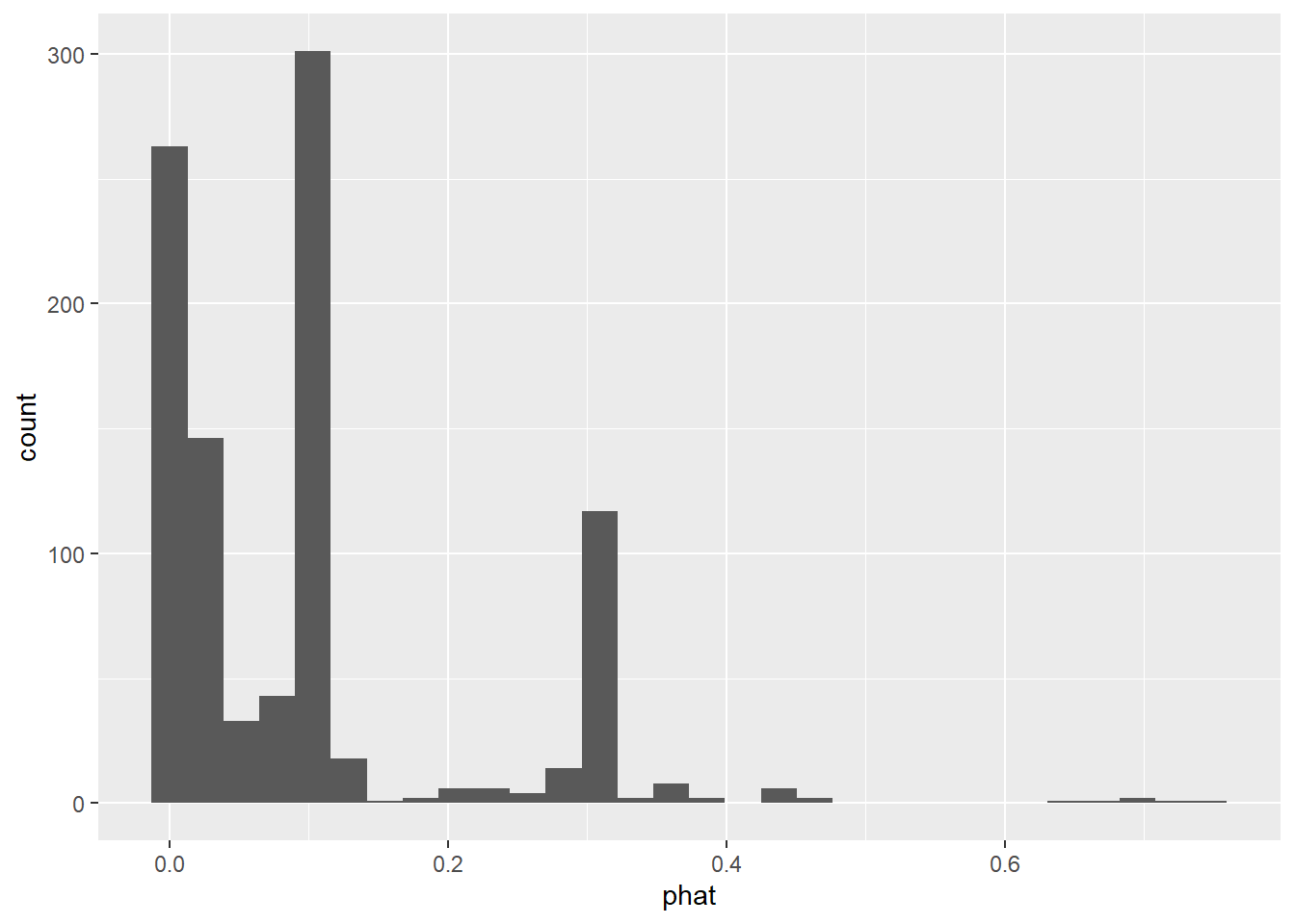

Before the highest phat was about .1. Here we’ve got a .8. That at least does predict some spam.

Now it looks like some of the predicted probabilities are fairly large, so let’s use the same classification rule we did above and recalculate MSPE:

ytilde <- ifelse(email25$phat >= 0.5,1,0)
(MSPE2 <- mean((ytilde-(as.integer(email25$spam)-1))^2))

[1] 0.09285714

Well…only a moderately better MSPE, but maybe we need a better classification rule. This is where looking at the ROC curve can help. We have a prediction model, and now we want to find the optimal classification rule.

ROC Curves

We’ll use the package pROC, so if you don’t have that installed you’ll have to get it.

# library(pROC)
# ?roc

roc(email25$spam,email25$phat,plot=TRUE)

Setting levels: control = 0, case = 1

Setting direction: controls < cases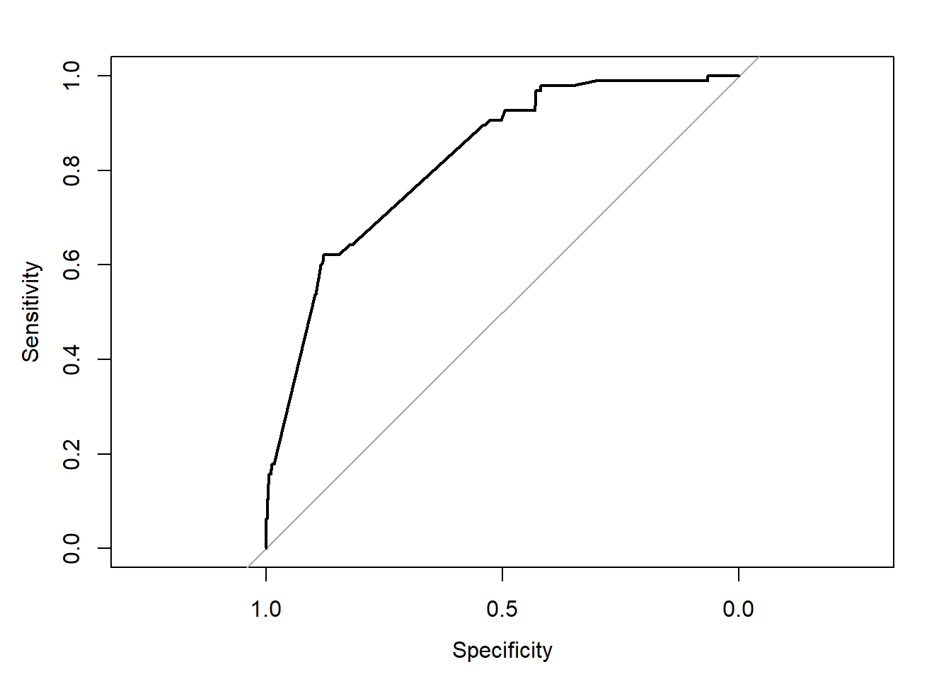


Call:
roc.default(response = email25$spam, predictor = email25$phat,     plot = TRUE)

Data: email25$phat in 885 controls (email25$spam 0) < 95 cases (email25$spam 1).
Area under the curve: 0.8214

Specificity instead of fpr on the x axis flips the numbers to high to low. Sensitivity is == tpr.

Looking for a point where we min fpr and max tpr.

This seems to suggest that we use 0.60 as our cut-off for the classification rule:

ytilde2 <- ifelse(email25$phat > 0.6,1,0)
(MSPE3 <- mean((ytilde2-(as.integer(email25$spam)-1))^2))

[1] 0.09285714

This is just marginally better than our original cut-off of 0.5, but we’re not going to get much better using this prediction model.

Next Steps

In the lab for this module, you’ll look at finding other prediction models for the email data that might do a better job than this one did.

Cross Validation

k-fold cross validation and more than two categories.

training and test sets are for cross validation.
As in LR MSE, GLM MSPE is similar
for k fold we split the data into k samples of roughly equal size.

When we split into 25:75 test:training. MSPE was .082.

using cv.glm in the boot package we can do k-fold.
for k = 10, we get .084, and for k = 5 it’s the same.

The real power comes from comparing models.

comparing models by k = 10 shows the number of preds and MSPE going up together.
Still need to consider parsimony and overfitting.

For more than 2 categories, like spam, not spam, and maybe.

we need training data for this type of prediction.
we would use multinomial log regs which is a generalization of binary logistic reg.
or we could use machine learning.

Big Data Issues

Big p and big n

p is number of exp variables. n is the number of observations.

big is in terms of p and n.
genomics might have n = 10 and p = 200,000. That’s big data.
weather over 30 years of monthly weather in 1km^2 grid can be terabytes.

When p is large compared to n.

if p => n you should not fit a model, it will fit exactly.
if p < n but close, there is still likely overfitting.
don’t use all the preds, but model selection then becomes a process.
Many of the same issues occur with cat vars.

When n is large:

bigger sample doesn’t mean better.
large n won’t improve inference if non-random
won’t improve ability to make causal inference without randomization to treatments.
won’t solve dependency issues.
won’t solve missing data issues if non-random.

You can’t overcome lack of randomization. Randomness is more important than size.

With large n, small effects can be statistically significant.
Consider practical vs statistical significance.
lm and glm require the data to be in memory.
there are ways to swap out data and do it anyway.

Increasing sample size is often accompanied by increasingly complicated relationships. This is more a conceptual problem that it is computational. It’s hard for us to think about complicated relationships.

The data must be informative about the thing we are interested in, having more data won’t help if it’s the wrong data.

Steps to looking at big data

look at a sample.
find a way to get a more representative set out of the whole to look at your question of interest.
analysis of a random sample can be used to make inference about the whole and the population.
summarize some aspects of the data, but be careful about the perils of aggregation.

If you see a summary table created from any dataset, large or small, be sure to consider whether the counts in the table have been aggregated over another factor or set of factors and if those had been included, would the information in the summary be different?

Working with big data in R

This is 1 hour long. I am not going to try and do the whole thing here. I’ll just watch it later.

Lab and HW

# Shows the factor dummy coding. 
contrasts(crashi2$Time.Cat)

Quiz R

The first two questions rely on the email dataset from the openintro package. Use the following R code to get set up for answering the questions below.

library(openintro)
data(email)
m1 <- glm(spam ~ to_multiple, data = email, family = "binomial")
m2 <- glm(spam ~ winner, data = email, family = "binomial")

1

Based on these two model fits, which is larger, the estimated probability of spam when the e-mail contains the word “winner” or the estimated probability of spam when the e-mail was sent to only one recipient?

summary(m1)


Call:
glm(formula = spam ~ to_multiple, family = "binomial", data = email)

Coefficients:
             Estimate Std. Error z value Pr(>|z|)    
(Intercept)  -2.11609    0.05618 -37.665  < 2e-16 ***
to_multiple1 -1.80918    0.29685  -6.095  1.1e-09 ***
---
Signif. codes:  0 '***' 0.001 '**' 0.01 '*' 0.05 '.' 0.1 ' ' 1

(Dispersion parameter for binomial family taken to be 1)

    Null deviance: 2437.2  on 3920  degrees of freedom
Residual deviance: 2372.0  on 3919  degrees of freedom
AIC: 2376

Number of Fisher Scoring iterations: 6

exp(-2.11609 - 1.80918)

[1] 0.01973681

summary(m2)


Call:
glm(formula = spam ~ winner, family = "binomial", data = email)

Coefficients:
            Estimate Std. Error z value Pr(>|z|)    
(Intercept) -2.31405    0.05627 -41.121  < 2e-16 ***
winneryes    1.52559    0.27549   5.538 3.06e-08 ***
---
Signif. codes:  0 '***' 0.001 '**' 0.01 '*' 0.05 '.' 0.1 ' ' 1

(Dispersion parameter for binomial family taken to be 1)

    Null deviance: 2437.2  on 3920  degrees of freedom
Residual deviance: 2412.7  on 3919  degrees of freedom
AIC: 2416.7

Number of Fisher Scoring iterations: 5

exp(-2.31405 + 1.52559)

[1] 0.4545443

The estimated probability of spam when the email was sent to only one recipient

The estimated probability of spam when the email contained the word “winner.”

There is not enough information to tell from these two model fits.

2

Using a classification rule that says: Classify as one if p̂ ≥ 0.5, and classify as zero otherwise, how would you expect m1 and m2 to perform relative to each other as a spam classifier? Group of answer choices

predictions <- predict(m1, email, type = "link")
phats <- plogis(predictions)

preds <- ifelse(phats >= 0.5, 1, 0)
(MSPE <- mean((as.integer(email$spam) - preds -1)^2))

[1] 0.09359857

predictions <- predict(m2, email, type = "link")
phats <- plogis(predictions)

preds <- ifelse(phats >= 0.5, 1, 0)
(MSPE <- mean((as.integer(email$spam) - preds -1)^2))

[1] 0.09359857

m1 should out-perform m2.

m2 should out-perform m1.

They should perform the same.

There is no way to tell.

3

Which of the following best describes the K argument to the cv.glm function? Group of answer choices

This is the number of bootstrap re-samples that are made.

None of these.

This is the size of the hold-out groups for cross validation.

This is the number of groups into which the data are split for cross validation.

4

Run the following code in R and examine the summary.

set.seed(10345)
Y <- rbinom(1000000, 1,0.3)
X <- rnorm(1000000, 0,1)
out <- glm (Y~X, family = binomial)
summary (out)


Call:
glm(formula = Y ~ X, family = binomial)

Coefficients:
             Estimate Std. Error  z value Pr(>|z|)    
(Intercept) -0.850609   0.002184 -389.538  < 2e-16 ***
X           -0.005947   0.002185   -2.722  0.00649 ** 
---
Signif. codes:  0 '***' 0.001 '**' 0.01 '*' 0.05 '.' 0.1 ' ' 1

(Dispersion parameter for binomial family taken to be 1)

    Null deviance: 1220552  on 999999  degrees of freedom
Residual deviance: 1220545  on 999998  degrees of freedom
AIC: 1220549

Number of Fisher Scoring iterations: 4

What can you conclude here?

Group of answer choices

All of these.

This is just a fluke—whoever created this code picked just the right set.seed value.

There is strong evidence (p = 0.006) that X and Y are associated

This is an example where the big-ness of the data is driving the statistical significance.

None of these.

Quiz C

1

Suppose you obtain a prediction from a Poisson regression model and a negative binomial regression model. Both predictions are 27.4, but the one from the Poisson model has an associated standard error of 3.4 while the one from the negative binomial model has a standard error of 5.2. Which prediction is better?

The one with the smaller standard error—better precision!
It doesn’t matter since they both give the same prediction.
The one with the larger standard error since it is more likely to accurately reflect the underlying variation in the data.
It depends on how the prediction is going to be used.
a and b

f. c and d

2

True or False? You can have a good predictive model and a poor classification rule.

True

False

There is not enough information to know.

3

Consider the ROC curve shown below. Choose the classification rule that would (approximately) do the best job at simultaneously maximizing specificity and sensitivity.

If p̂ ≥ 0.30 then classify as a one, otherwise classify as a zero

If p̂ ≥ 0.63 then classify as a one, otherwise classify as a zero.

If p̂ ≥ 0.75 then classify as a one, otherwise classify as a zero

It’s impossible to tell.

4

Why is randomly sampling cases from a big dataset and then performing statistical modeling on the sampled data a reasonable approach?

Because the random sampling ensures that you get a representative sample from the large dataset.

You shouldn’t do this, because you will lose the power of the big dataset.

You shouldn’t do this, beacuse you can just apply the regular modeling tools to the large dataset.